# A tibble: 1 × 1
   mean
  <dbl>
1 174.Summarizing data, a Review
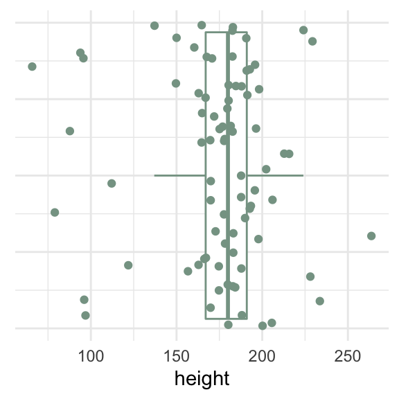
One continuous variable
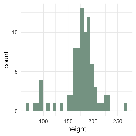
How can we visualize a single continuous variable?
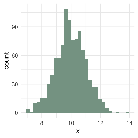
Histogram
Code
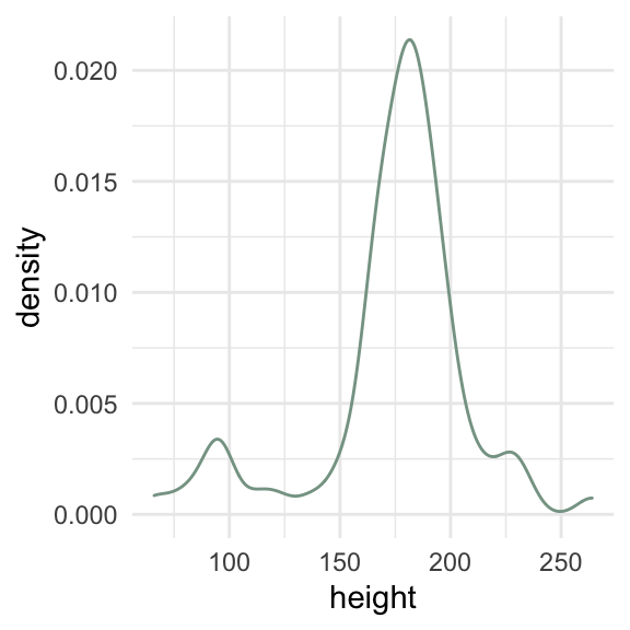
Density
One continuous variable
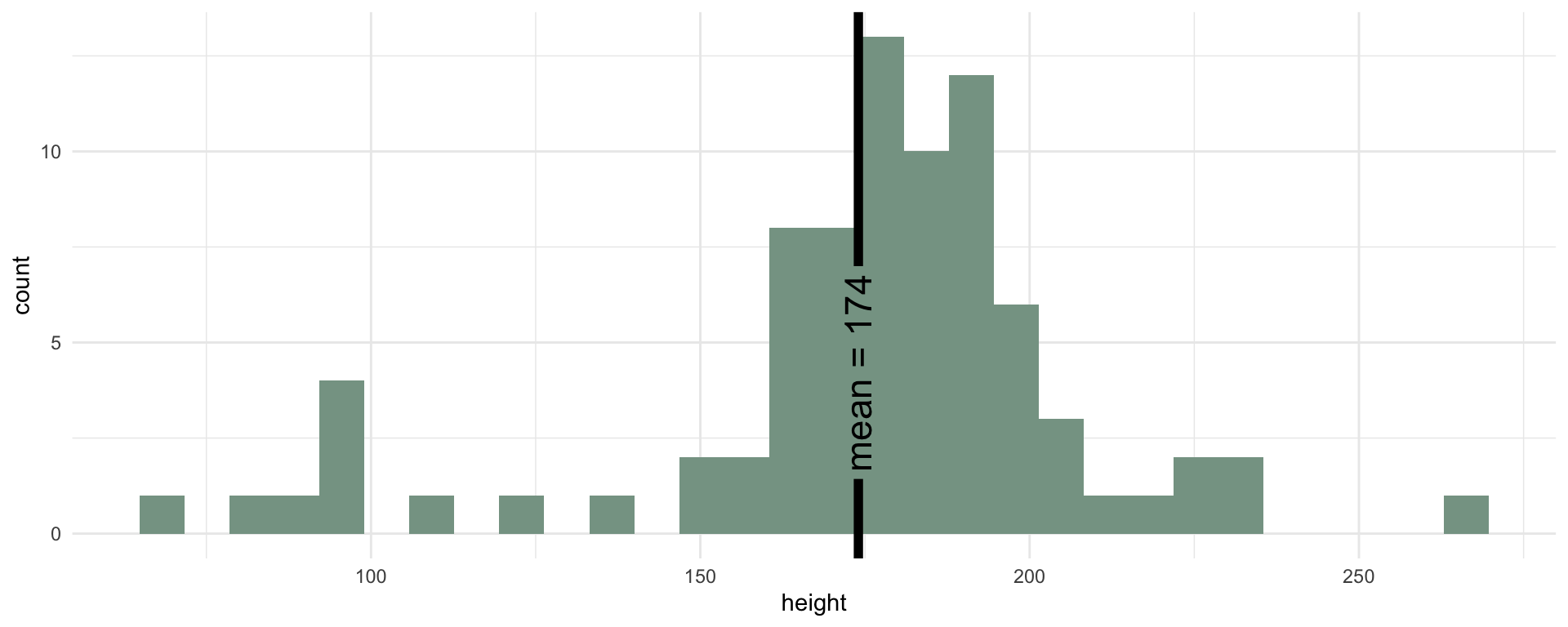
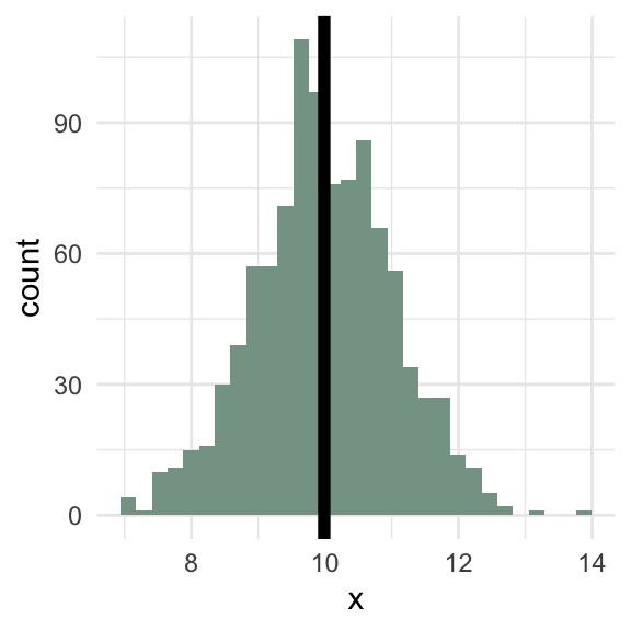
Meaningful means
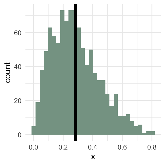
Symmetric
Code
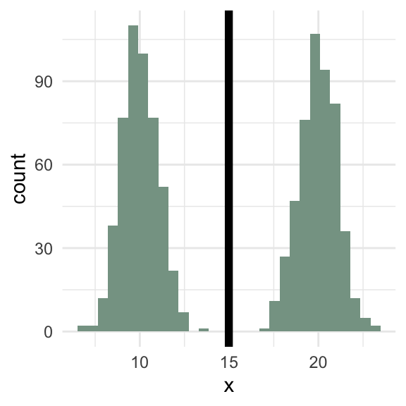
Bimodal
Code
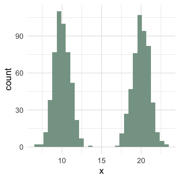
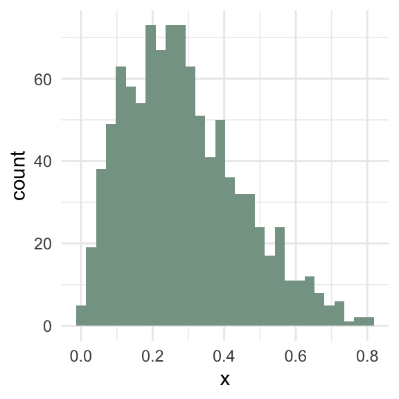
Guess the mean for each of these variables.
Meaningful means
Symmetric
Code
Bimodal
Code
Does this value represent a “typical” observation?
Data
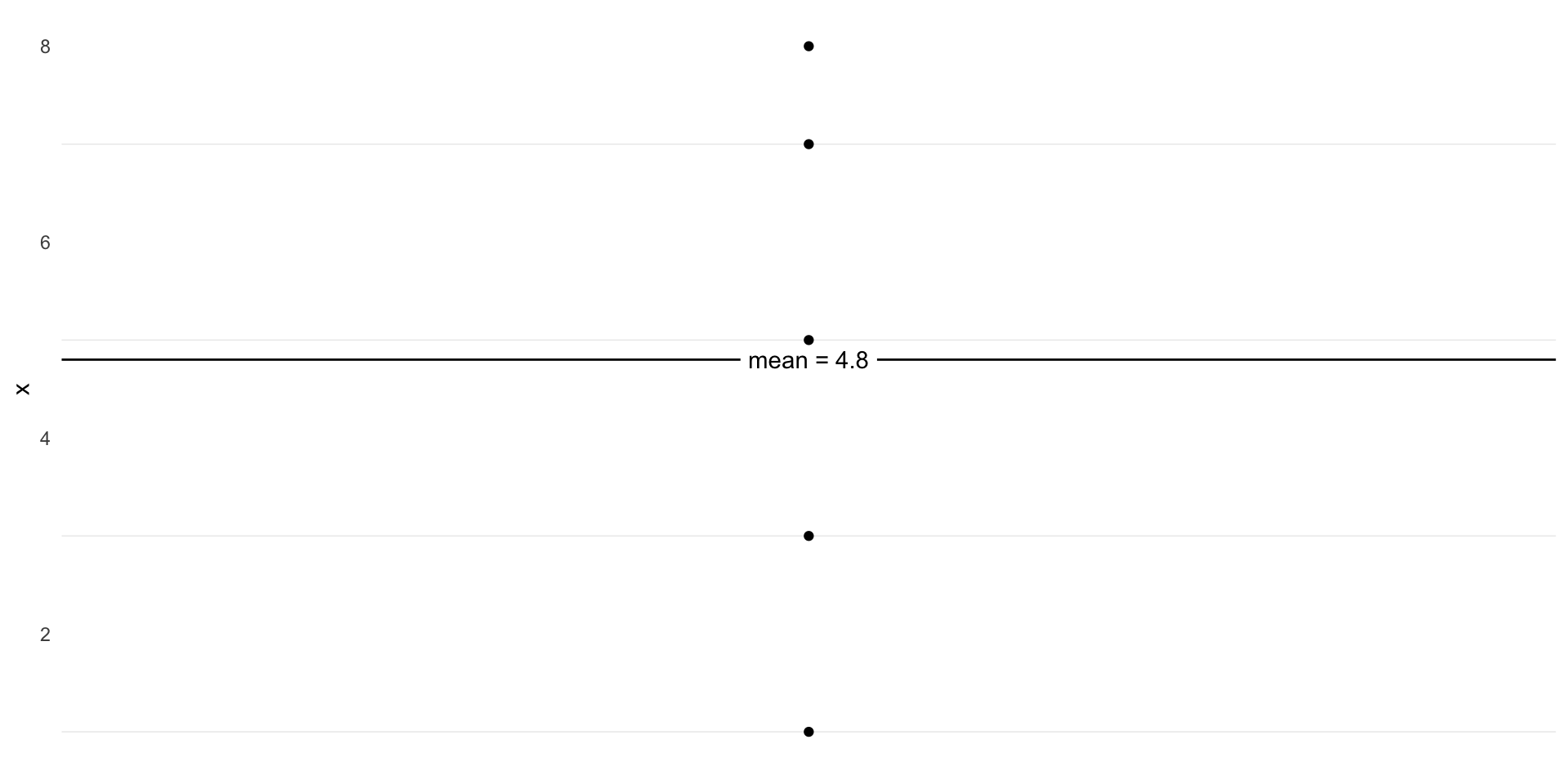
Data
Code
ggplot(d, aes(x = i, y = x)) +
  geom_point() +
  geom_texthline(yintercept = mean(d$x), label = "mean = 4.8") +
  geom_segment(aes(y = x, yend = mean(x), x = i, xend = i), color = "blue") +
  theme(axis.ticks.x = element_blank(),
        axis.title.x = element_blank(),
        axis.text.x = element_blank(),
        panel.grid.major = element_blank(),
        panel.grid.minor.x = element_blank())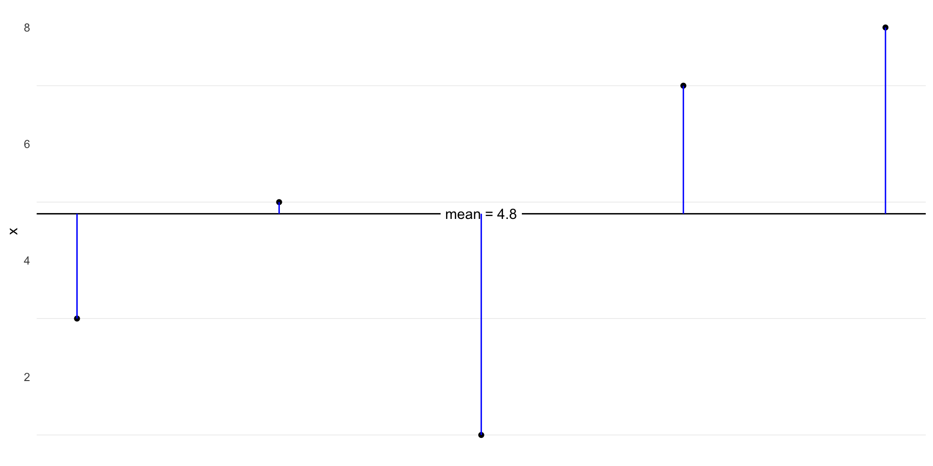
Data
Code
ggplot(d, aes(x = i, y = x)) +
  geom_point() +
  geom_texthline(yintercept = mean(d$x), lwd = 5, hjust = 0.1,
                 label = as.character(expression(beta[0])), parse = TRUE) +
  geom_segment(aes(y = x, yend = mean(x), x = i, xend = i), color = "blue") +
  theme(axis.ticks.x = element_blank(),
        axis.title.x = element_blank(),
        axis.text.x = element_blank(),
        panel.grid.major = element_blank(),
panel.grid.minor.x = element_blank()) 
Data
Code
ggplot(d, aes(x = i, y = x)) +
  geom_point() +
  geom_texthline(yintercept = mean(d$x), lwd = 5, hjust = 0.1,
                 label = as.character(expression(beta[0])), parse = TRUE) +
  geom_textsegment(aes(y = x, yend = mean(x), x = i, xend = i), color = "blue",
                   label = as.character(expression(epsilon)), parse = TRUE,
                   lwd = 5) +
  theme(axis.ticks.x = element_blank(),
        axis.title.x = element_blank(),
        axis.text.x = element_blank(),
        panel.grid.major = element_blank(),
        panel.grid.minor.x = element_blank())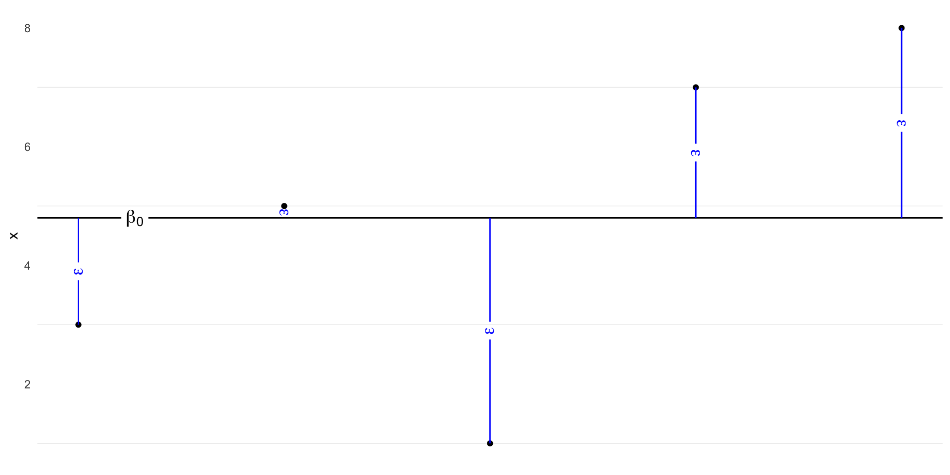
Data
Code
ggplot(d, aes(x = 1, y = x)) +
  geom_point() +
  geom_texthline(yintercept = mean(d$x), lwd = 5, hjust = 0.1,
                 label = as.character(expression(beta[0])), parse = TRUE) +
  geom_segment(aes(y = x, yend = mean(x), x = 1, xend = 1), color = "blue") +
  theme(axis.ticks.x = element_blank(),
        axis.title.x = element_blank(),
        axis.text.x = element_blank(),
        panel.grid.major = element_blank(),
panel.grid.minor.x = element_blank()) 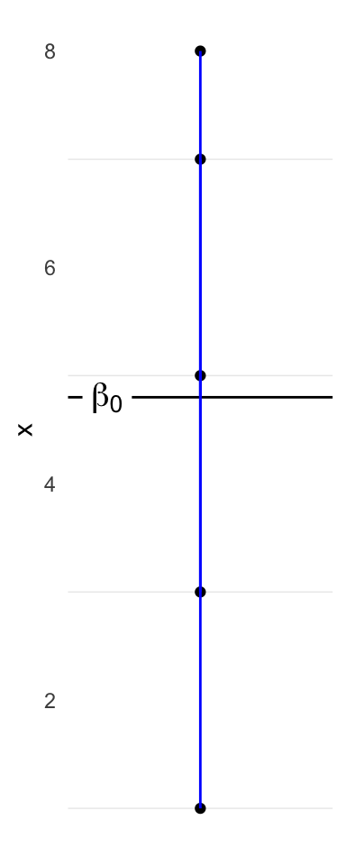
Data
Code
ggplot(d, aes(x = 1, y = x)) +
  geom_point() +
  geom_texthline(yintercept = mean(d$x), lwd = 5, hjust = 0.1,
                 label = as.character(expression(beta[0])), parse = TRUE) +
  geom_segment(aes(y = x, yend = mean(x), x = 1, xend = 1), color = "blue") +
  theme(axis.ticks.x = element_blank(),
        axis.title.x = element_blank(),
axis.text.x = element_blank()) 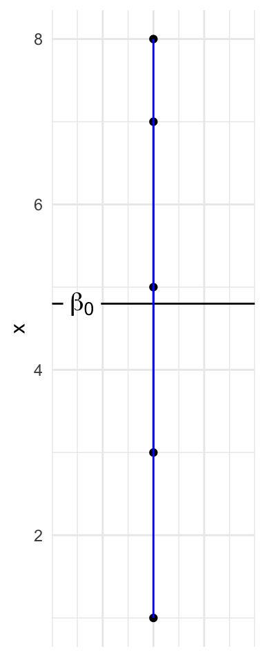
Recap
When is the mean an appropriate summary measure to calculate?
What assumptions need to be true in order to use a mean to represent your single continuous variable?
