Simple Linear Regression Part 2
Simple linear regression
How did we decide on this line?
Code
starwars_nojabba <- starwars_nojabba %>%
  mutate(fitted = fitted(lm(mass ~ height, data = starwars_nojabba)))

ggplot(starwars_nojabba, aes(x = height, mass)) +
  geom_point(color = "#86a293") +
  geom_segment(aes(
    x = height,
    y = mass,
    xend = height,
    yend = fitted
  ),
  color = "blue") +
  geom_smooth(
    method = "lm",
    se = FALSE,
    formula = "y ~ x",
    color = "#86a293"
  ) +
  labs(title = "The relationship between mass and height for Star Wars characters",
       caption = "Data from SWAPI (swapi.dev)")
Minimize Least Squares
Code
ggplot(starwars_nojabba, aes(x = height, mass)) +
  geom_rect(
    aes(
      xmin = height,
      xmax = height + mass - fitted,
      ymin = mass,
      ymax = fitted
    ),
    fill = "blue",
    color = "blue",
    alpha = 0.2
  ) +
  geom_smooth(
    method = "lm",
    se = FALSE,
    formula = "y ~ x",
    color = "#86a293"
  ) +
  geom_point(color = "#86a293") +
  coord_fixed() +
  labs(title = "The relationship between mass and height for Star Wars characters",
       caption = "Data from SWAPI (swapi.dev)")
“Squared Residuals”
Code
ggplot(starwars_nojabba, aes(x = height, mass)) +
  geom_rect(
    aes(
      xmin = height,
      xmax = height + mass - fitted,
      ymin = mass,
      ymax = fitted
    ),
    fill = "blue",
    color = "blue",
    alpha = 0.2
  ) +
  geom_smooth(
    method = "lm",
    se = FALSE,
    formula = "y ~ x",
    color = "#86a293"
  ) +
  geom_point(color = "#86a293") +
  coord_fixed() +
  labs(title = "The relationship between mass and height for Star Wars characters",
       caption = "Data from SWAPI (swapi.dev)")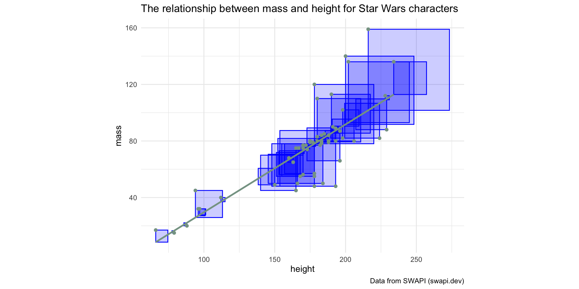
“Residuals”
Code
ggplot(starwars_nojabba, aes(x = height, mass)) +
  geom_point(color = "#86a293") +
  geom_segment(aes(
    x = height,
    y = mass,
    xend = height,
    yend = fitted
  ),
  color = "blue") +
  geom_smooth(
    method = "lm",
    se = FALSE,
    formula = "y ~ x",
    color = "#86a293"
  ) +
  labs(title = "The relationship between mass and height for Star Wars characters",
       caption = "Data from SWAPI (swapi.dev)")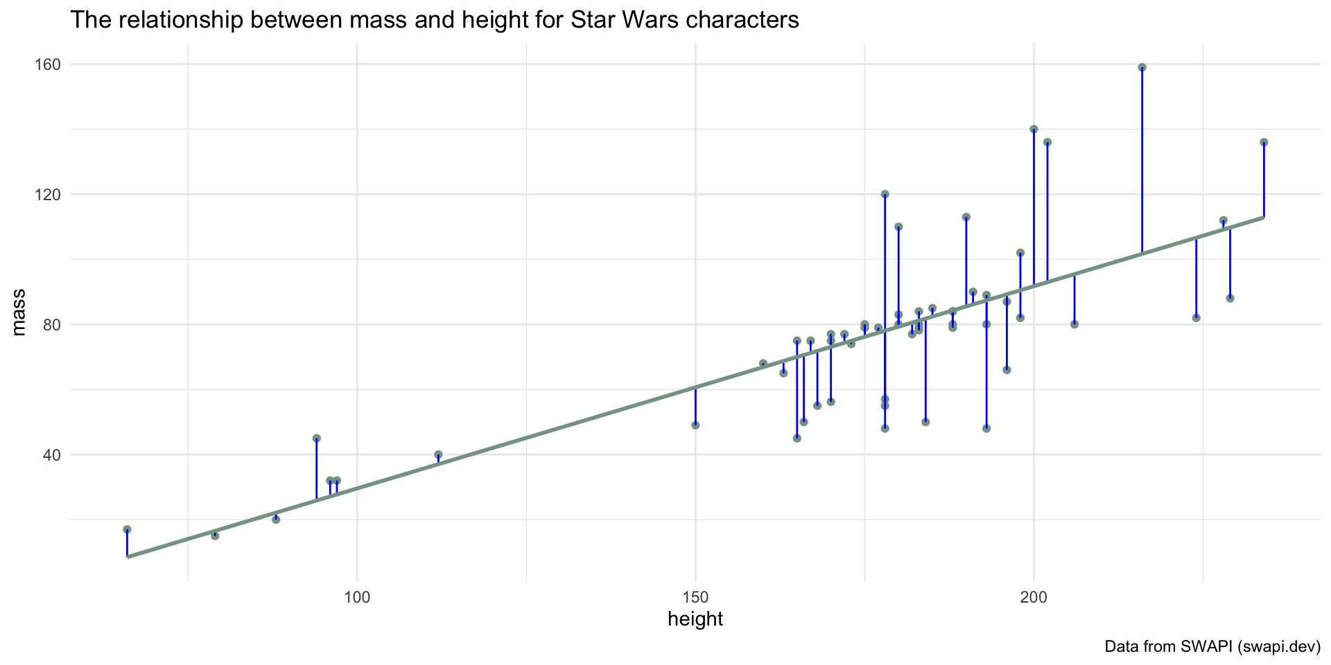
Application Exercise
- Create a new project from this template in RStudio Pro:
- Load the packages and data by running the top chunk of R code
- Learn about the
PorschePricedata by running?PorschePricein your Console - Fit a linear model predicting
PricefromMileage - Add a variable called
y_hatto thePorschePricedataset with the predicted y values - Add a variable called
residualto thePorschePricedataset with the residuals
07:00
