Drawing Inference

Lucy D’Agostino McGowan

Data

magnolia_data 

# A tibble: 30 × 3
   observation leaf_length leaf_width
         <dbl>       <dbl>      <dbl>
 1          21        10.4        4.4
 2          19        21          9  
 3          15        26         11  
 4           4        17.8        6.4
 5          23        15         10  
 6          15        15          8  
 7          26        18         13  
 8          14        19          6  
 9          22        29.3       14.6
10           7        14.2        8.8
# … with 20 more rows

When is a simple linear regression model a useful descriptive summary?

• Linearity holds
• The residuals have “zero mean” (this is always true!)
• The datapoints are independent

What if we want to draw inference on another sample?

Inference

• So far we’ve only been able to describe our sample
• For example, we’ve just been describing \(\hat{\beta}_1\) the estimated slope of the relationship between \(x\) and \(y\)
• What if we want to extend these claims to the population?

Magnolia data

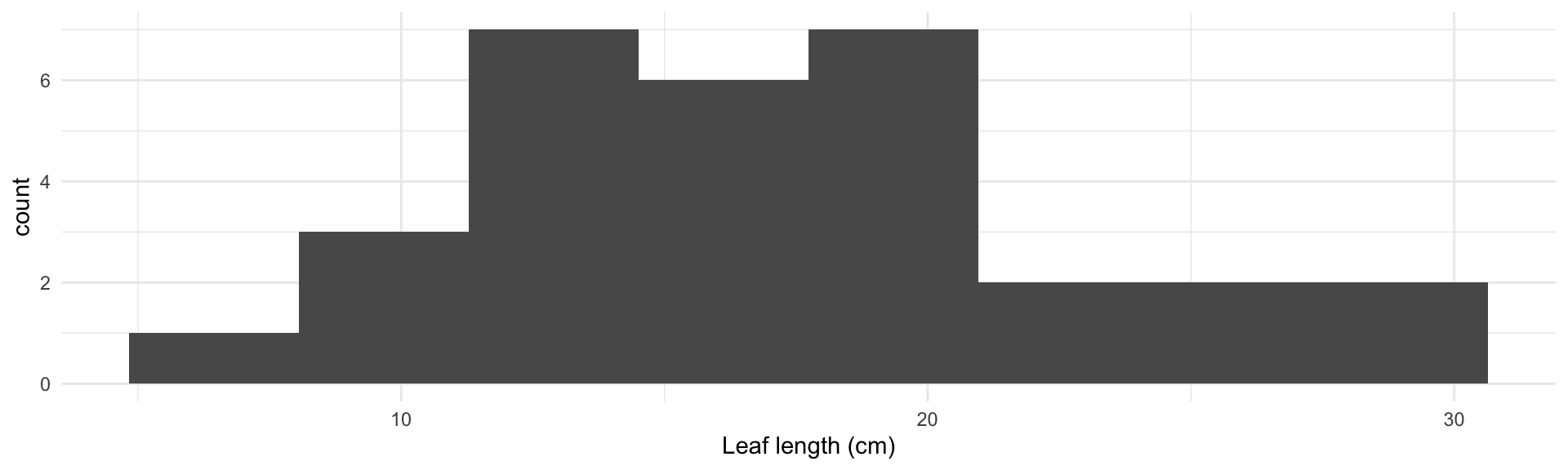
How can I visualize a single continuous variable?

Code

ggplot(magnolia_data, aes(x = leaf_length)) +
  geom_histogram(bins = 8) + 
  labs(x = "Leaf length (cm)")

Magnolia data

Code

set.seed(1)
ggplot(full_magnolia_data, 
       aes(x = leaf_length, y = 1)) + 
  geom_boxplot() + 
  geom_jitter() + 
  labs(x = "Leaf length (cm)") +
  theme(axis.title.y = element_blank(),
        axis.text.y = element_blank(),
        axis.ticks.y = element_blank())

Magnolia data

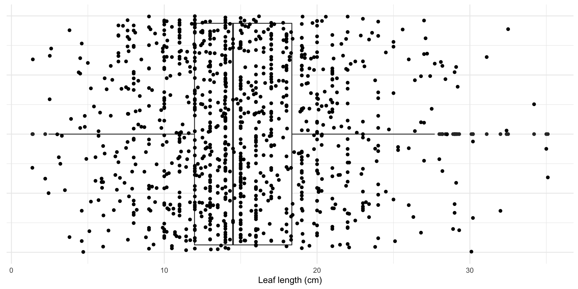
Code

set.seed(1)

ggplot(full_magnolia_data, 
       aes(x = leaf_length, y = 1)) + 
  geom_boxplot() + 
  geom_jitter() + 
  geom_jitter(data = magnolia_data, color = "cornflower blue", size = 3) + 
  labs(x = "Leaf length (cm)") +
  theme(axis.title.y = element_blank(),
        axis.text.y = element_blank(),
        axis.ticks.y = element_blank())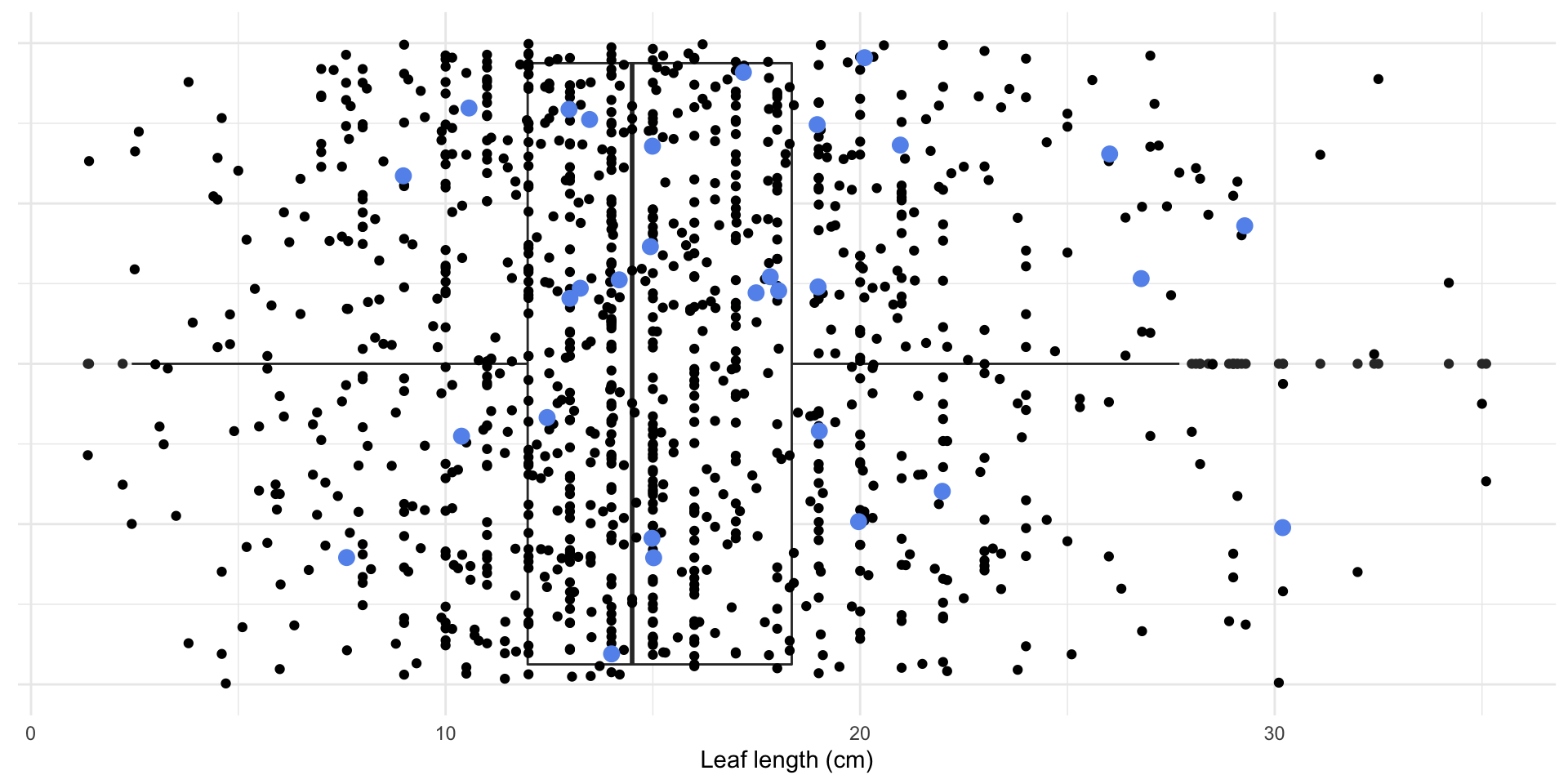

Magnolia data

Code

set.seed(1)

ggplot(full_magnolia_data,
       aes(x = leaf_length, 
           y = in_sample,
           color = in_sample)) + 
  geom_boxplot() + 
  geom_jitter() + 
  scale_color_manual(values = c("black", "cornflower blue")) + 
  theme(legend.position = "none") + 
  labs(x = "Leaf length (cm)",
       y = "in sample")

Magnolia data

How can I calculate the average leaf length of the magnolias in my sample in R?

magnolia_data %>%
  summarize(mean_length = mean(leaf_length))

# A tibble: 1 × 1
  mean_length
        <dbl>
1        17.1

lm(leaf_length ~ 1, data = magnolia_data)

Call:
lm(formula = leaf_length ~ 1, data = magnolia_data)

Coefficients:
(Intercept)  
      17.13  

Magnolia data

What if I want to know the average leaf length of the magnolias on the Mag Quad?

How can we quantify how much we’d expect the mean to differ from one random sample to another?

• We need a measure of uncertainty
• How about the standard error of the mean?
• The standard error is how much we expect the sample mean to vary from one random sample to another.

Magnolia data

How can we quantify how much we’d expect the mean to differ from one random sample to another?

mod <- lm(leaf_length ~ 1, data = magnolia_data)
summary(mod)

Call:
lm(formula = leaf_length ~ 1, data = magnolia_data)

Residuals:
   Min     1Q Median     3Q    Max 
-9.509 -3.809 -1.029  2.621 13.071 

Coefficients:
            Estimate Std. Error t value Pr(>|t|)    
(Intercept)   17.129      1.031   16.62 2.32e-16 ***
---
Signif. codes:  0 '***' 0.001 '**' 0.01 '*' 0.05 '.' 0.1 ' ' 1

Residual standard error: 5.645 on 29 degrees of freedom

Application Exercise

1. Create a new project from this template in RStudio Pro:

https://github.com/sta-112-f22/appex-08.git

2. Replace the text in the top code chunk that says INSERT YOUR GOOGLE SPREADSHEET URL HERE with the Google Spreadsheet URL with your magnolia data.
3. Fit an intercept only model to calculate the average leaf length in your sample
4. Use the summary function on the linear model you fit
5. What is the standard error for the mean length? Interpret this value.

05:00

confidence intervals

If we use the same sampling method to select different samples and computed an interval estimate for each sample, we would expect the true population parameter (the average leaf length on the Mag Quad) to fall within the interval estimates 95% of the time.

Confidence interval

\[\bar{x} \pm t^∗ \times SE_{\bar{x}}\]

• \(t^*\) is the critical value for the \(t_{n−1}\) density curve to obtain the desired confidence level
• Often we want a 95% confidence level.

Demo

Let’s do it in R!

mod <- lm(leaf_length ~ 1, data = magnolia_data)
summary(mod) 

Call:
lm(formula = leaf_length ~ 1, data = magnolia_data)

Residuals:
   Min     1Q Median     3Q    Max 
-9.509 -3.809 -1.029  2.621 13.071 

Coefficients:
            Estimate Std. Error t value Pr(>|t|)    
(Intercept)   17.129      1.031   16.62 2.32e-16 ***
---
Signif. codes:  0 '***' 0.001 '**' 0.01 '*' 0.05 '.' 0.1 ' ' 1

Residual standard error: 5.645 on 29 degrees of freedom

qt(0.025, df = nrow(magnolia_data) - 1, lower.tail = FALSE)

[1] 2.04523

Let’s do it in R!

Why 0.025?

mod <- lm(leaf_length ~ 1, data = magnolia_data)
summary(mod) 

Call:
lm(formula = leaf_length ~ 1, data = magnolia_data)

Residuals:
   Min     1Q Median     3Q    Max 
-9.509 -3.809 -1.029  2.621 13.071 

Coefficients:
            Estimate Std. Error t value Pr(>|t|)    
(Intercept)   17.129      1.031   16.62 2.32e-16 ***
---
Signif. codes:  0 '***' 0.001 '**' 0.01 '*' 0.05 '.' 0.1 ' ' 1

Residual standard error: 5.645 on 29 degrees of freedom

qt(0.025, df = nrow(magnolia_data) - 1, lower.tail = FALSE)

[1] 2.04523

Let’s do it in R!

Why lower.tail = FALSE?

mod <- lm(leaf_length ~ 1, data = magnolia_data)
summary(mod) 

Call:
lm(formula = leaf_length ~ 1, data = magnolia_data)

Residuals:
   Min     1Q Median     3Q    Max 
-9.509 -3.809 -1.029  2.621 13.071 

Coefficients:
            Estimate Std. Error t value Pr(>|t|)    
(Intercept)   17.129      1.031   16.62 2.32e-16 ***
---
Signif. codes:  0 '***' 0.001 '**' 0.01 '*' 0.05 '.' 0.1 ' ' 1

Residual standard error: 5.645 on 29 degrees of freedom

qt(0.025, df = nrow(magnolia_data) - 1, lower.tail = FALSE)

[1] 2.04523

Let’s do it in R!

mod <- lm(leaf_length ~ 1, data = magnolia_data)
summary(mod) 

Call:
lm(formula = leaf_length ~ 1, data = magnolia_data)

Residuals:
   Min     1Q Median     3Q    Max 
-9.509 -3.809 -1.029  2.621 13.071 

Coefficients:
            Estimate Std. Error t value Pr(>|t|)    
(Intercept)   17.129      1.031   16.62 2.32e-16 ***
---
Signif. codes:  0 '***' 0.001 '**' 0.01 '*' 0.05 '.' 0.1 ' ' 1

Residual standard error: 5.645 on 29 degrees of freedom

t_star <- qt(0.025, df = nrow(magnolia_data) - 1, lower.tail = FALSE)
14.827 + t_star * 0.912

[1] 16.7

14.827 - t_star * 0.912

[1] 13

confint(mod) 

            2.5 % 97.5 %
(Intercept)    15   19.2

confidence intervals

If we use the same sampling method to select different samples and computed an interval estimate for each sample, we would expect the true population parameter (the mean) to fall within the interval estimates 95% of the time.

Application Exercise

1. Open appex-08.qmd
2. Calculate the \(t^*\) value for your confidence interval
3. Calculate the confidence interval “by hand” using the \(t^*\) value from exercise 2 and the mean and standard error from the previous application exercise
4. Calculate the confidence interval using the confint function
5. Interpret this value

05:00