Drawing Inference
Lucy D’Agostino McGowan
Data
Magnolia data
Full Magnolia data
full_magnolia_data <- full_magnolia_data %>%
  group_by(id) %>%
  summarise(max_length = max(leaf_length),
            min_length = min(leaf_length),
            mean_length = mean(leaf_length),
            mean_width = mean(leaf_width)) %>%
  mutate(inches = ifelse(max_length < 10, 1, 0),
         inches = ifelse(min_length < 2, 1, 0),
         flipped = ifelse(mean_length < mean_width, 1, 0)) %>%
  left_join(full_magnolia_data, by = "id") %>%
  select(-max_length, -mean_length, - mean_width) %>%
  mutate(leaf_length2 = ifelse(flipped, leaf_width, leaf_length),
         leaf_width = ifelse(flipped, leaf_length, leaf_width),
         leaf_length = leaf_length2)
Magnolia data
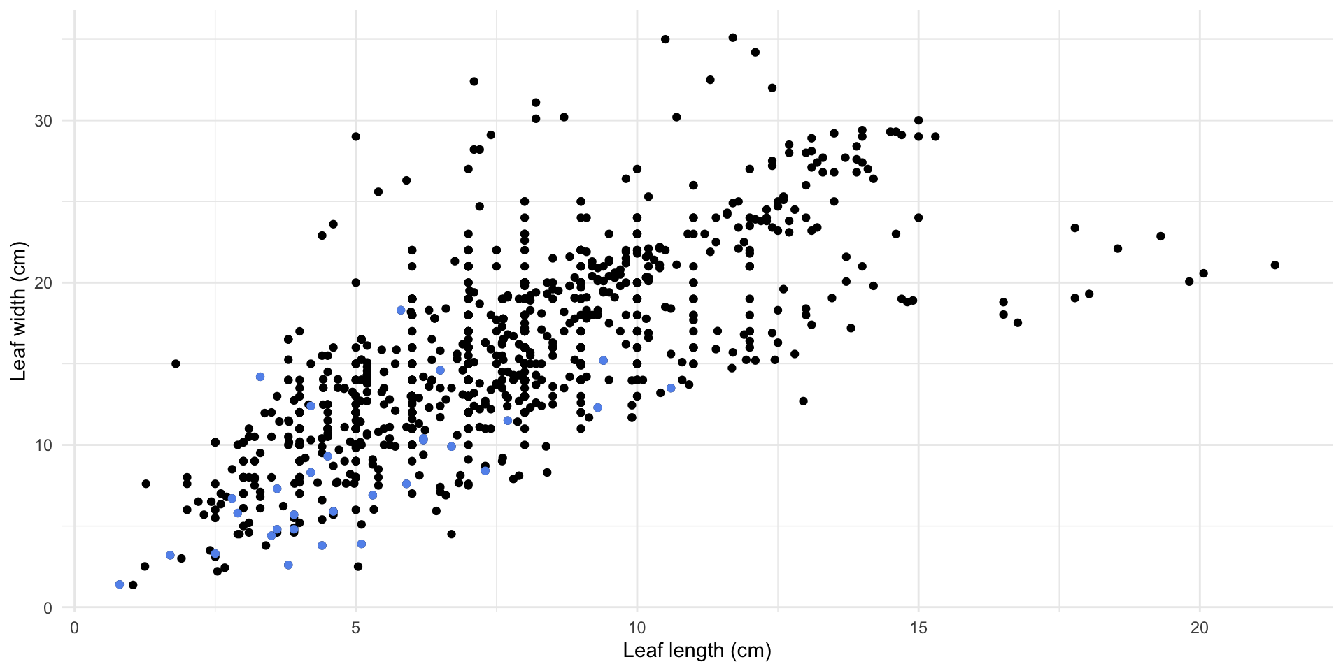
Magnolia data
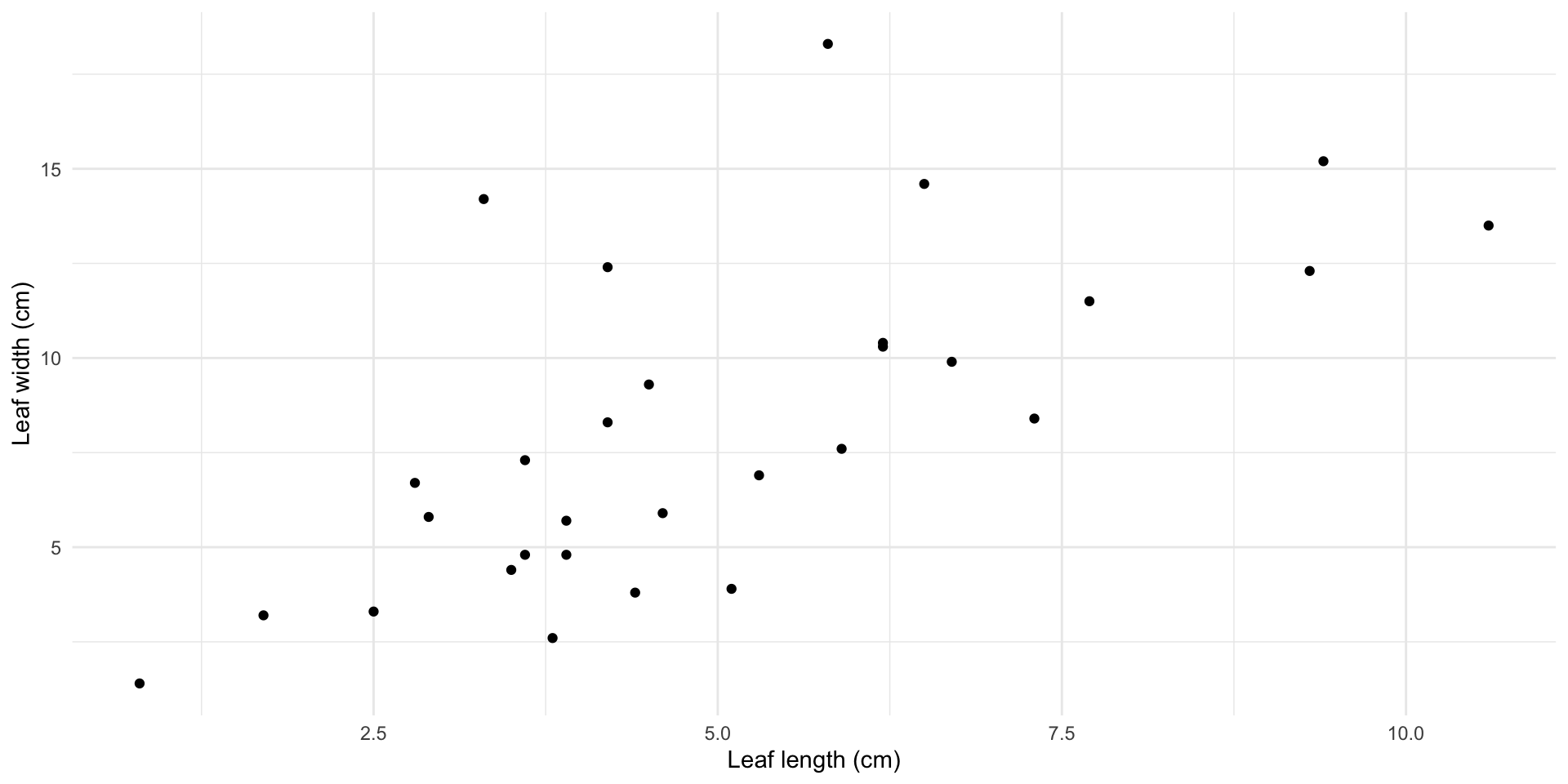
What if I want to know the relationship between leaf length and leaf width of the magnolias on the Mag Quad?
How can we quantify how much we’d expect the slope to differ from one random sample to another?
- We need a measure of uncertainty
- How about the standard error of the slope?
- The standard error is how much we expect \(\hat{\beta}_1\) to vary from one random sample to another.
Magnolia data
How can we quantify how much we’d expect the slope to differ from one random sample to another?
Call:
lm(formula = leaf_length ~ leaf_width, data = magnolia_data)

Residuals:
    Min      1Q  Median      3Q     Max
-4.4424 -1.7942 -0.9585  1.0470  9.0647

Coefficients:
            Estimate Std. Error t value Pr(>|t|)
(Intercept)   1.8369     1.4507   1.266    0.216
leaf_width    1.2756     0.2645   4.822 4.51e-05 ***
---
Signif. codes:  0 '***' 0.001 '**' 0.01 '*' 0.05 '.' 0.1 ' ' 1

Residual standard error: 3.243 on 28 degrees of freedom
Multiple R-squared:  0.4537,    Adjusted R-squared:  0.4342
F-statistic: 23.26 on 1 and 28 DF,  p-value: 4.507e-05
Magnolia data
We need a test statistic that incorporates \(\hat{\beta}_1\) and the standard error
Call:
lm(formula = leaf_length ~ leaf_width, data = magnolia_data)

Residuals:
    Min      1Q  Median      3Q     Max
-4.4424 -1.7942 -0.9585  1.0470  9.0647

Coefficients:
            Estimate Std. Error t value Pr(>|t|)
(Intercept)   1.8369     1.4507   1.266    0.216
leaf_width    1.2756     0.2645   4.822 4.51e-05 ***
---
Signif. codes:  0 '***' 0.001 '**' 0.01 '*' 0.05 '.' 0.1 ' ' 1

Residual standard error: 3.243 on 28 degrees of freedom
Multiple R-squared:  0.4537,    Adjusted R-squared:  0.4342
F-statistic: 23.26 on 1 and 28 DF, p-value: 4.507e-05- \(t = \frac{\hat{\beta}_1}{SE_{\hat{\beta}_1}}\)
Magnolia data
How do we interpret this?
Call:
lm(formula = leaf_length ~ leaf_width, data = magnolia_data)

Residuals:
    Min      1Q  Median      3Q     Max
-4.4424 -1.7942 -0.9585  1.0470  9.0647

Coefficients:
            Estimate Std. Error t value Pr(>|t|)
(Intercept)   1.8369     1.4507   1.266    0.216
leaf_width    1.2756     0.2645   4.822 4.51e-05 ***
---
Signif. codes:  0 '***' 0.001 '**' 0.01 '*' 0.05 '.' 0.1 ' ' 1

Residual standard error: 3.243 on 28 degrees of freedom
Multiple R-squared:  0.4537,    Adjusted R-squared:  0.4342
F-statistic: 23.26 on 1 and 28 DF, p-value: 4.507e-05- “\(\hat{\beta}_1\) is more than 4.82 standard errors above a slope of zero”
Magnolia data
How do we know what values of this statistic are worth paying attention to?
Call:
lm(formula = leaf_length ~ leaf_width, data = magnolia_data)

Residuals:
    Min      1Q  Median      3Q     Max
-4.4424 -1.7942 -0.9585  1.0470  9.0647

Coefficients:
            Estimate Std. Error t value Pr(>|t|)
(Intercept)   1.8369     1.4507   1.266    0.216
leaf_width    1.2756     0.2645   4.822 4.51e-05 ***
---
Signif. codes:  0 '***' 0.001 '**' 0.01 '*' 0.05 '.' 0.1 ' ' 1

Residual standard error: 3.243 on 28 degrees of freedom
Multiple R-squared:  0.4537,    Adjusted R-squared:  0.4342
F-statistic: 23.26 on 1 and 28 DF, p-value: 4.507e-05- confidence intervals
- p-values
- Hypothesis testing: \(H_0: \beta_1 = 0\) \(H_A: \beta_1 \neq 0\)
Magnolia data
How do get a confidence interval for \(\hat{\beta}_1\)? What function can we use in R?
How do we interpret this value?
Application Exercise
- Open
appex-08.qmd - Fit the model of
leaf_lengthandleaf_widthin your data - Calculate a confidence interval for the estimate \(\hat\beta_1\)
- Interpret this value
05:00
Hypothesis testing
- So far, we have estimated the relationship between the length of magnolia leaves and the width.
- This could be useful if we wanted to understand, on average, how these variables are related (estimation)
- This could also be useful if we wanted to guess how long a leaf was based on how wide it is (prediction)
- What if we just want to know whether there is some relationship bewteen the two? (hypothesis testing)
Hypothesis testing
- Null hypothesis: There is no relationship between leaf length and leaf width
- \(H_0: \beta_1 = 0\)
- Alternative hypothesis: There is a relationship between leaf length and leaf width
- \(H_A: \beta_1 \neq 0\)
Hypothesis testing
Call:
lm(formula = leaf_length ~ leaf_width, data = magnolia_data)

Residuals:
    Min      1Q  Median      3Q     Max
-4.4424 -1.7942 -0.9585  1.0470  9.0647

Coefficients:
            Estimate Std. Error t value Pr(>|t|)
(Intercept)   1.8369     1.4507   1.266    0.216
leaf_width    1.2756     0.2645   4.822 4.51e-05 ***
---
Signif. codes:  0 '***' 0.001 '**' 0.01 '*' 0.05 '.' 0.1 ' ' 1

Residual standard error: 3.243 on 28 degrees of freedom
Multiple R-squared:  0.4537,    Adjusted R-squared:  0.4342
F-statistic: 23.26 on 1 and 28 DF,  p-value: 4.507e-05
Is \(\hat\beta_1\) different from 0?
Hypothesis testing
Call:
lm(formula = leaf_length ~ leaf_width, data = magnolia_data)

Residuals:
    Min      1Q  Median      3Q     Max
-4.4424 -1.7942 -0.9585  1.0470  9.0647

Coefficients:
            Estimate Std. Error t value Pr(>|t|)
(Intercept)   1.8369     1.4507   1.266    0.216
leaf_width    1.2756     0.2645   4.822 4.51e-05 ***
---
Signif. codes:  0 '***' 0.001 '**' 0.01 '*' 0.05 '.' 0.1 ' ' 1

Residual standard error: 3.243 on 28 degrees of freedom
Multiple R-squared:  0.4537,    Adjusted R-squared:  0.4342
F-statistic: 23.26 on 1 and 28 DF,  p-value: 4.507e-05
Is \(\beta_1\) different from 0? (notice the lack of the hat!)
p-value
The probability of observing a statistic as extreme or more extreme than the observed test statistic given the null hypothesis is true
p-value
Call:
lm(formula = leaf_length ~ leaf_width, data = magnolia_data)

Residuals:
    Min      1Q  Median      3Q     Max
-4.4424 -1.7942 -0.9585  1.0470  9.0647

Coefficients:
            Estimate Std. Error t value Pr(>|t|)
(Intercept)   1.8369     1.4507   1.266    0.216
leaf_width    1.2756     0.2645   4.822 4.51e-05 ***
---
Signif. codes:  0 '***' 0.001 '**' 0.01 '*' 0.05 '.' 0.1 ' ' 1

Residual standard error: 3.243 on 28 degrees of freedom
Multiple R-squared:  0.4537,    Adjusted R-squared:  0.4342
F-statistic: 23.26 on 1 and 28 DF,  p-value: 4.507e-05
What is the p-value? What is the interpretation?
Hypothesis testing
- Null hypothesis: \(\beta_1 = 0\) (there is no relationship between the width and length of a magnolia leaf)
- Alternative hypothesis: \(\beta_1 \neq 0\) (there is a relationship between the width and length of a magnolia leaf)
- Often we have an \(\alpha\) level cutoff to compare the p-value to, for example 0.05.
- If p-value < 0.05, we reject the null hypothesis
- If p-value > 0.05, we fail to reject the null hypothesis
- Why don’t we ever “accept” the null hypothesis?
- absense of evidence is not evidence of absense
p-value
Call:
lm(formula = leaf_length ~ leaf_width, data = magnolia_data)

Residuals:
    Min      1Q  Median      3Q     Max
-4.4424 -1.7942 -0.9585  1.0470  9.0647

Coefficients:
            Estimate Std. Error t value Pr(>|t|)
(Intercept)   1.8369     1.4507   1.266    0.216
leaf_width    1.2756     0.2645   4.822 4.51e-05 ***
---
Signif. codes:  0 '***' 0.001 '**' 0.01 '*' 0.05 '.' 0.1 ' ' 1

Residual standard error: 3.243 on 28 degrees of freedom
Multiple R-squared:  0.4537,    Adjusted R-squared:  0.4342
F-statistic: 23.26 on 1 and 28 DF,  p-value: 4.507e-05
Do we reject the null hypothesis?
Application Exercise
- Open
appex-08.qmd - Examine the summary of the model of
leaf_lengthandleaf_widthwith your data - Test the null hypothesis that there is no relationship between the length and width of magnolia leaves
- What is the p-value? What is the result of your hypothesis test?
02:00
