Unusual Observations
Lucy D’Agostino McGowan
Outlier
Points for which the magnitude of the residual is unusually large. These are points that are unusually far away from the overall pattern.
Influential point
Influential points exert considerable impact on the estimated regression line
Leverage
The leverage of a point dictates how much a point influences the slope of a fitted regression line. Points with high leverage pull the regression line in their direction.
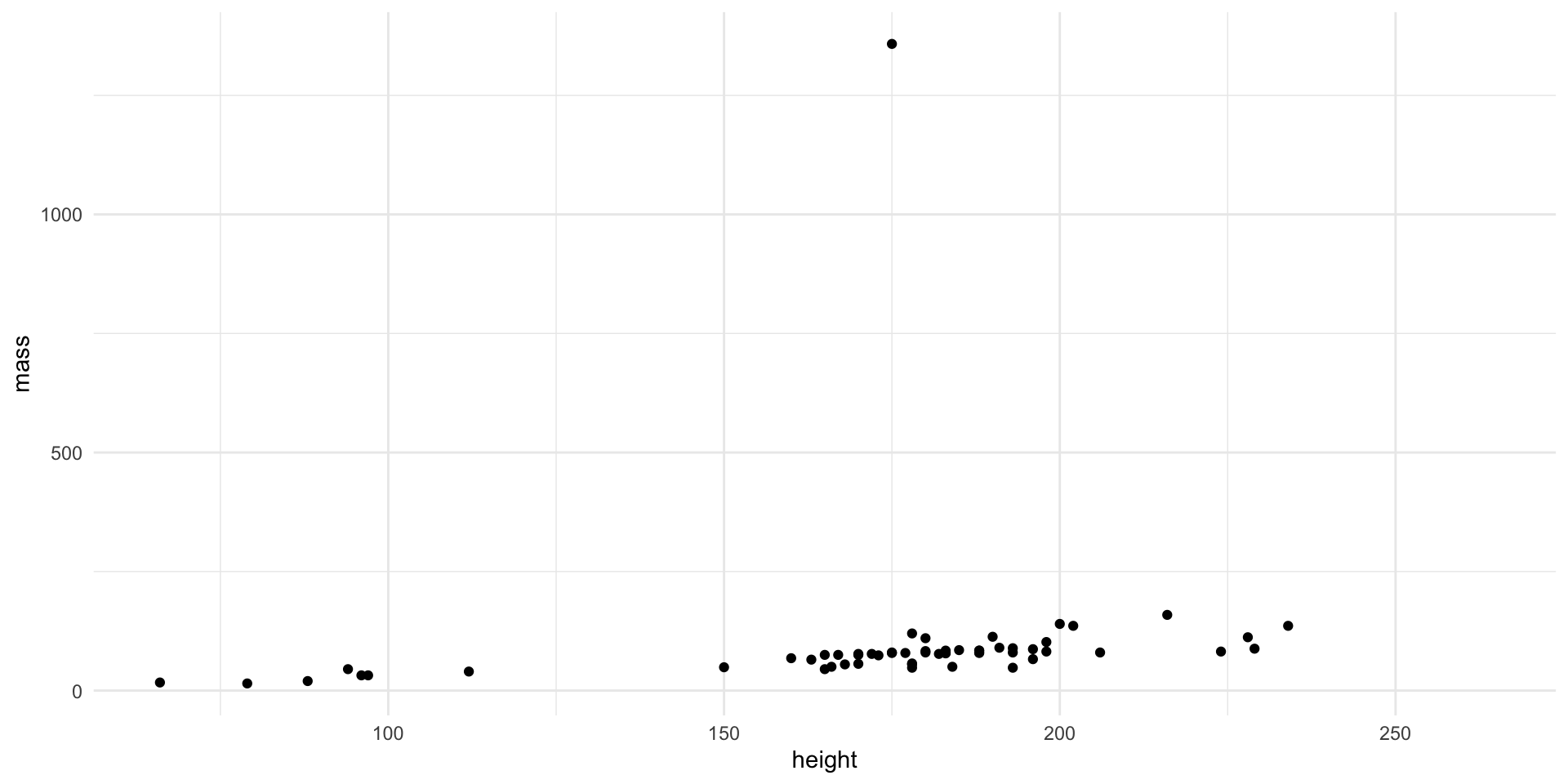
Example
Code
ggplot (starwars, aes (height, mass)) + geom_point ()
Example
lm (mass ~ height, data = starwars)
Call:
lm(formula = mass ~ height, data = starwars)

Coefficients:
(Intercept)       height
   -13.8103       0.6386
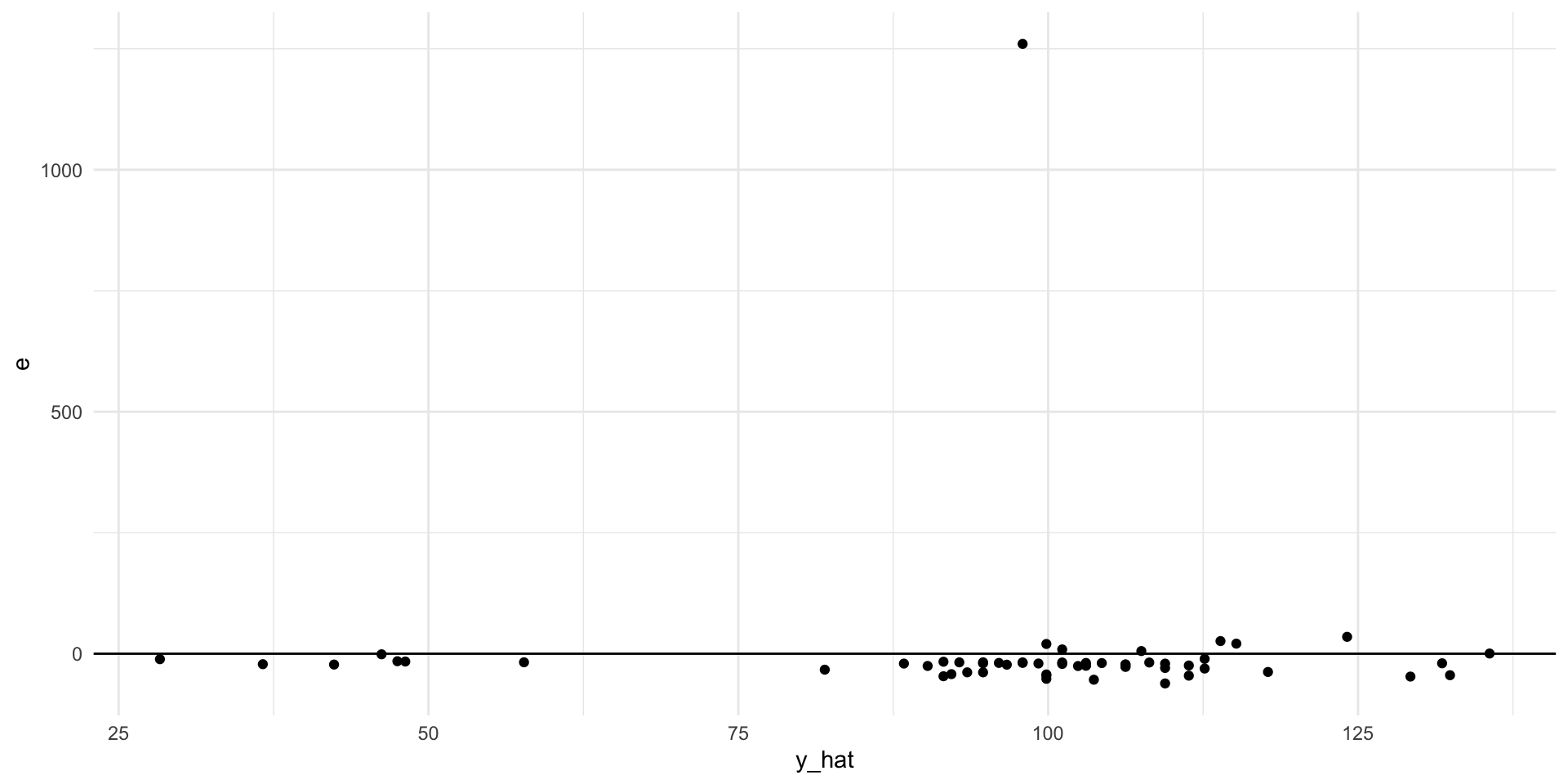
Example
<- lm (mass ~ height, data = starwars)%>% drop_na (height, mass) %>% mutate (y_hat = fitted (mod),e = residuals (mod)) %>% ggplot (aes (y_hat, e)) + geom_point () + geom_hline (yintercept = 0 )
Example
What does this line of code do?
<- lm (mass ~ height, data = starwars)%>% drop_na (height, mass) %>% mutate (y_hat = fitted (mod),e = residuals (mod)) %>% ggplot (aes (y_hat, e)) + geom_point () + geom_hline (yintercept = 0 )
Example
What does this line of code do?
<- lm (mass ~ height, data = starwars)%>% drop_na (height, mass) %>% mutate (y_hat = fitted (mod),e = residuals (mod)) %>% ggplot (aes (y_hat, e)) + geom_point () + geom_hline (yintercept = 0 )
Example
<- lm (mass ~ height,data = starwars)%>% drop_na (height, mass) %>% mutate (y_hat = fitted (mod),e = residuals (mod)) %>% ggplot (aes (y_hat, e)) + geom_point () + geom_hline (yintercept = 0 )
Example
Gold-medal-winning distances (m) for the men’s Olympic long jump, 1900–2008
library (Stat2Data)data ("LongJumpOlympics" )ggplot (LongJumpOlympics, aes (Year, Gold)) + geom_point ()
Example
Gold-medal-winning distances (m) for the men’s Olympic long jump, 1900–2008
Code
<- lm (Gold ~ Year, data = LongJumpOlympics)%>% mutate (y_hat = fitted (mod),e = residuals (mod)) %>% ggplot (aes (y_hat, e)) + geom_point () + geom_hline (yintercept = 0 ) + labs (x = "fitted" )
Example
Gold-medal-winning distances (m) for the men’s Olympic long jump, 1900–2008
Code
%>% mutate (y_hat = fitted (mod),e = residuals (mod)) %>% ggplot (aes (y_hat, e, color = e > 0.6 )) + geom_point () + geom_hline (yintercept = 0 ) + scale_color_manual (values = c ("black" , "red" )) + labs (x = "fitted" ) + theme (legend.position = "none" )
Example
<- lm (Gold ~ Year, data = LongJumpOlympics)
How can we tell if a residual is “unusually” large?
Do we have a “typical” error we can standardize by?
Standardized residuals
\(\hat{\sigma}_\varepsilon\) : reflects the typical error\(\Large\frac{\textrm{residual}}{\hat{\sigma}_\varepsilon}\) \(\Large{\frac{y - \hat{y}}{\hat{\sigma}_\varepsilon}}\)
Standardized residuals
\(\hat{\sigma}_\varepsilon\) : reflects the typical error\(\Large\frac{\textrm{residual}}{\hat{\sigma}_\varepsilon}\) \(\Large{\frac{y - \hat{y}}{\hat{\sigma}_\varepsilon}}\)
%>% mutate (e = residuals (mod)) %>% summarise (sigma = sqrt (sum (e^ 2 ) / (n () - 2 )
Standardized residuals
\(\hat{\sigma}_\varepsilon\) : reflects the typical error\(\Large\frac{\textrm{residual}}{\hat{\sigma}_\varepsilon}\) \(\Large{\frac{y - \hat{y}}{\hat{\sigma}_\varepsilon}}\)
%>% mutate (e = residuals (mod)) %>% summarise (sigma = sqrt (sum (e^ 2 ) / (n () - 2 )
Standardized residuals
\(\hat{\sigma}_\varepsilon\) : reflects the typical error\(\Large\frac{\textrm{residual}}{\hat{\sigma}_\varepsilon}\) \(\Large{\frac{y - \hat{y}}{\hat{\sigma}_\varepsilon}}\)
%>% mutate (stand_resid = residuals (mod) / sigma (mod))
   Year  Gold stand_resid
1  1900 7.185 -0.23644575
2  1904 7.340  0.17933378
3  1906 7.200 -0.52866109
4  1908 7.480  0.53194885
5  1912 7.600  0.80034465
6  1920 7.150 -1.56842880
7  1924 7.445 -0.56311433
8  1928 7.730  0.40009050
9  1932 7.640 -0.21581611
10 1936 8.060  1.31586884
11 1948 7.825 -0.38446725
12 1952 7.570 -1.69518289
13 1956 7.830 -0.83725216
14 1960 8.120  0.14700749
15 1964 8.070 -0.30046056
16 1968 8.900  2.95771956
17 1972 8.240 -0.05843643
18 1976 8.350  0.16784973
19 1980 8.540  0.73101299
20 1984 8.540  0.49409313
21 1988 8.720  1.01514676
22 1992 8.670  0.56767870
23 1996 8.500 -0.38510501
24 2000 8.550 -0.41147668
25 2004 8.590 -0.47995799
26 2008 8.370 -1.64328990
Studentized residuals
Another option is to estimate the standard deviation of the regression error using a model that is fit after omitting the point in question
In R: rstudent()
Example
%>% mutate (stud_resid = rstudent (mod))
   Year  Gold  stud_resid
1  1900 7.185 -0.24969110
2  1904 7.340  0.18773767
3  1906 7.200 -0.55459469
4  1908 7.480  0.55605557
5  1912 7.600  0.83801927
6  1920 7.150 -1.69661296
7  1924 7.445 -0.57565964
8  1928 7.730  0.40587196
9  1932 7.640 -0.21761617
10 1936 8.060  1.37486325
11 1948 7.825 -0.38535068
12 1952 7.570 -1.80894501
13 1956 7.830 -0.84888005
14 1960 8.120  0.14690763
15 1964 8.070 -0.30102045
16 1968 8.900  3.76651449
17 1972 8.240 -0.05865636
18 1976 8.350  0.16903844
19 1980 8.540  0.74709891
20 1984 8.540  0.50367210
21 1988 8.720  1.05875652
22 1992 8.670  0.58546175
23 1996 8.500 -0.39790914
24 2000 8.550 -0.42816057
25 2004 8.590 -0.50378890
26 2008 8.370 -1.85376067
Example
%>% mutate (stud_resid = rstudent (mod)) %>% ggplot (aes (Year, stud_resid)) + geom_point () + geom_hline (yintercept = c (2 , 4 , - 2 , - 4 ), lty = 2 ) + labs (y = "studentized residual" )
Recap
Outliers are points that are unusually far from the overall pattern of the other dataYou can check for outliers by examining the residuals
One common rule of thumb is to “studentize” the residuals and look for ones that are smaller than -2 or larger than 2 and identify these as outliers
Influential points
Would removing the observation from the dataset change the regression equation by much?
Example
lm (mass ~ height, data = starwars)
Call:
lm(formula = mass ~ height, data = starwars)

Coefficients:
(Intercept)       height
   -13.8103       0.6386
%>% filter (name != "Jabba Desilijic Tiure" ) %>% lm (mass ~ height, data = .)
Call:
lm(formula = mass ~ height, data = .)

Coefficients:
(Intercept)       height
   -32.5408       0.6214
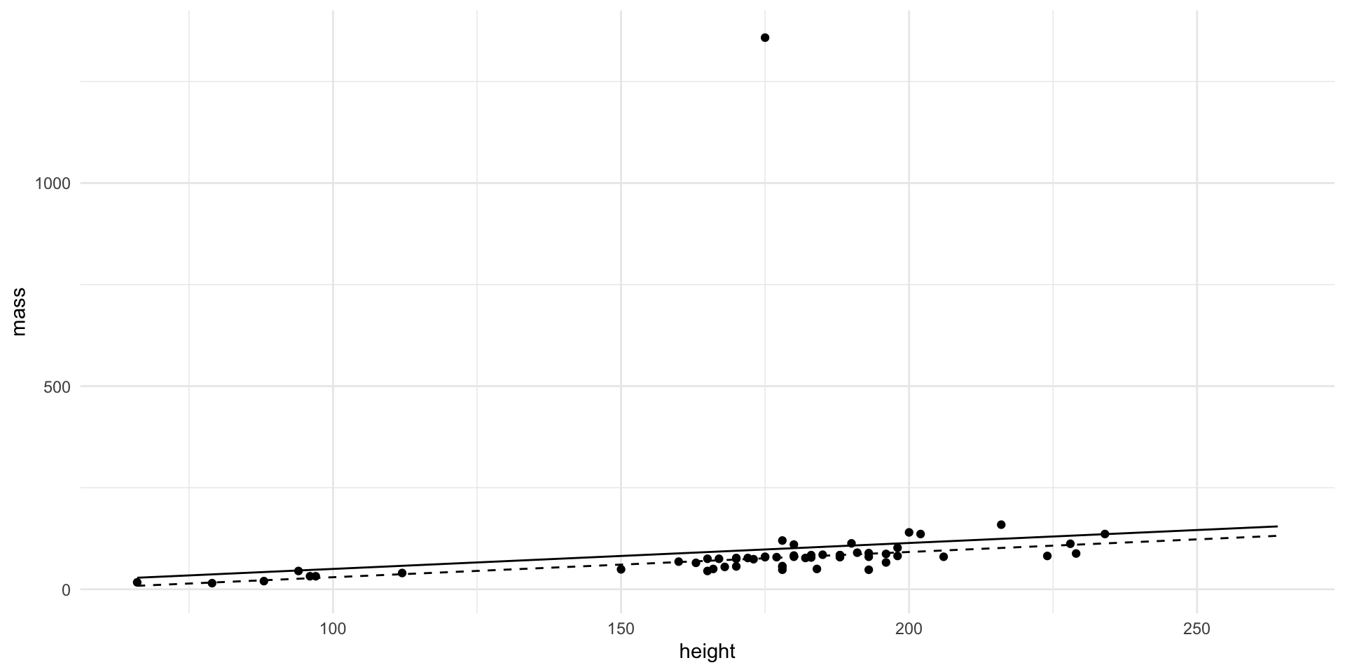
Example
Code
ggplot (starwars, aes (height, mass)) + geom_point () + geom_line (aes (height, - 13.8103 + 0.6386 * height)) + geom_line (aes (height, - 32.5408 + 0.6214 * height), lty = 2 )
Recap
Influential points change the overall regression line fitTo see if a point is influential fit the model with and without that point to see if the coefficients change
In general, points that are farther from the average value of the predictor value have a greater potential to influence the regression line
Application Exercise
Create a new project from this template in RStudio Pro:
https://github.com/sta-112-f22/appex-10.git
Load the packages and data by running the top chunk of R code
Learn about the USstamps data by running ?USstamps in your Console
Use the filter function to remove observations with Year less than 1958
Fit a linear model predicting the stamp price from year
Calculate the studentized residuals and plot them – are there any outliers?
If you found an outlier, refit the model without it – is this point “influential”?