Hypothesis Testing and P-values
Under the null hypothesis
Under the null \((\beta_1 = 0)\) the t-statistic \((\hat\beta_1/se_{\hat\beta_1})\) has a t-distribution with \(n-2\) degrees of freedom.
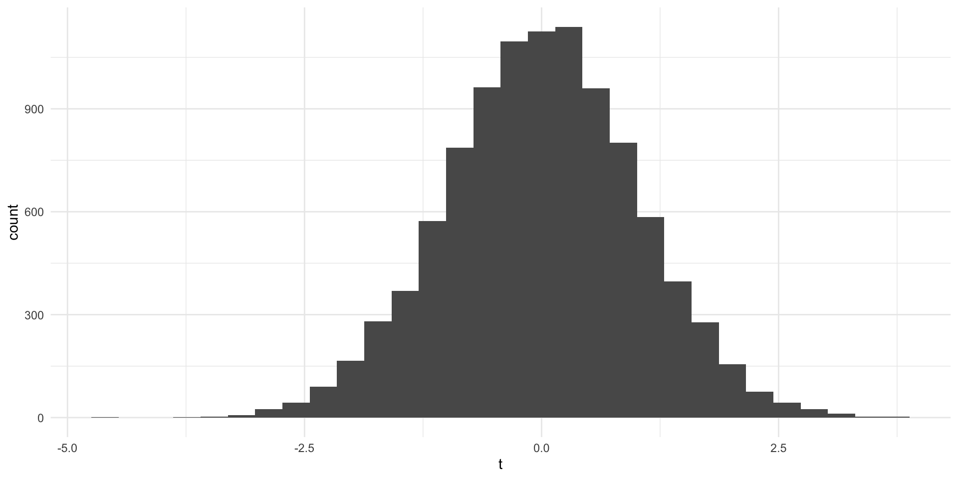
Under the Null Hypothesis
- How do we compare these to the distribution under the null?
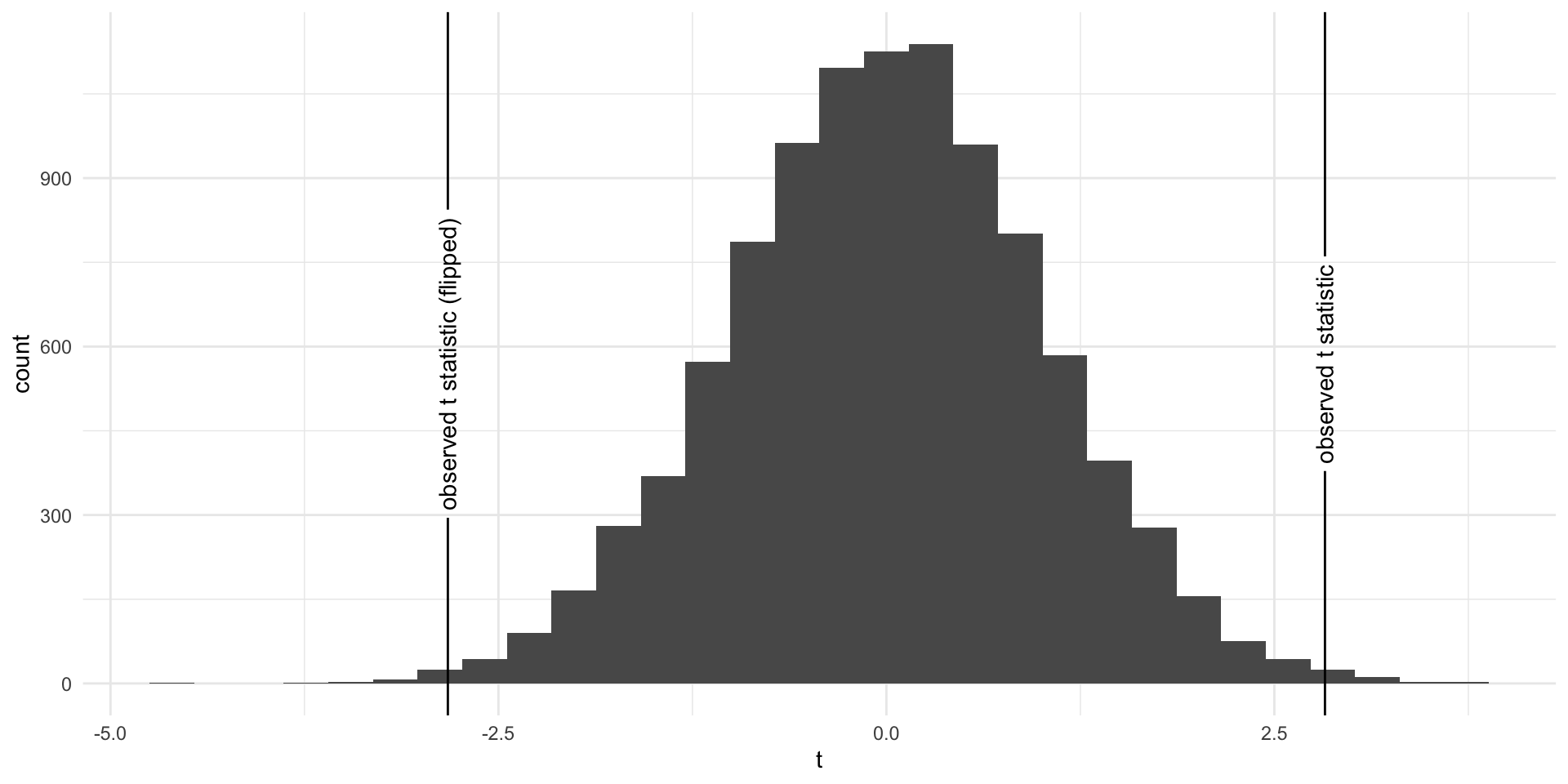
Under the Null Hypothesis
Code
null$color <- ifelse(null$t < 2.826 & null$t > -2.826, "out", "in")
ggplot(null, aes(t, fill = color)) +
  geom_histogram(bins = 30) +
  geom_textvline(xintercept = c(2.826), label = "observed t statistic") +
  geom_textvline(xintercept = c(-2.826), label = "observed t statistic (flipped)") +
  theme(legend.position = "none")
Under the Null Hypothesis
The proportion of area greater than 2.826
Code
null$color <- ifelse(null$t < 2.826 & null$t > -2.826, "out", "in")
ggplot(null, aes(t, fill = color)) +
  geom_histogram(bins = 30) +
  geom_textvline(xintercept = c(2.826), label = "observed t statistic") +
  geom_textvline(xintercept = c(-2.826), label = "observed t statistic (flipped)") +
  theme(legend.position = "none")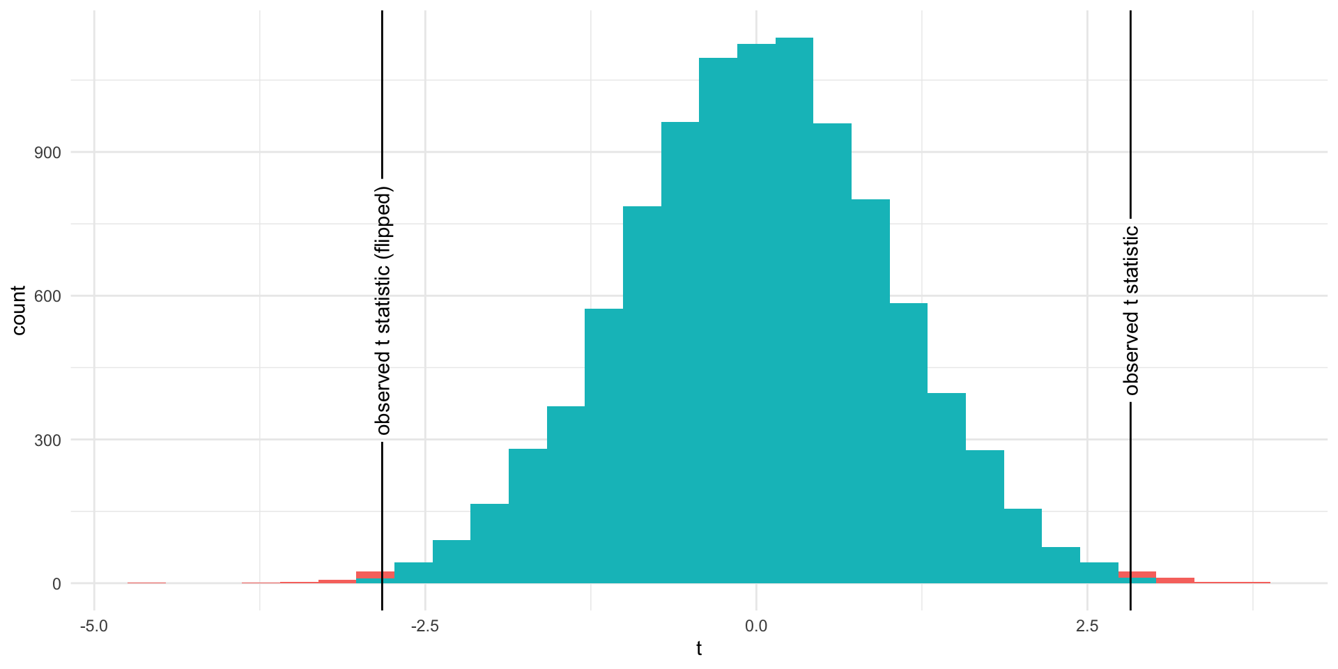
Under the Null Hypothesis
The proportion of area less than -2.826
Code
null$color <- ifelse(null$t < 2.826 & null$t > -2.826, "out", "in")
ggplot(null, aes(t, fill = color)) +
  geom_histogram(bins = 30) +
  geom_textvline(xintercept = c(2.826), label = "observed t statistic") +
  geom_textvline(xintercept = c(-2.826), label = "observed t statistic (flipped)") +
  theme(legend.position = "none")
Under the Null Hypothesis
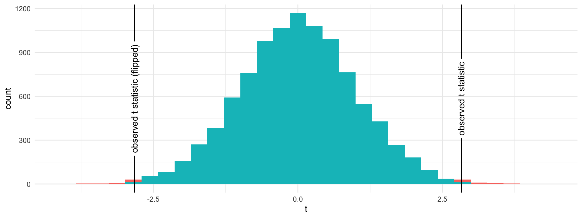
The proportion of area greater than 2.826 or less than -2.826
Code
null$color <- ifelse(null$t < 2.826 & null$t > -2.826, "out", "in")
ggplot(null, aes(t, fill = color)) +
  geom_histogram(bins = 30) +
  geom_textvline(xintercept = c(2.826), label = "observed t statistic") +
  geom_textvline(xintercept = c(-2.826), label = "observed t statistic (flipped)") +
  theme(legend.position = "none")
Under the Null Hypothesis
The proportion of area greater than 2.826 or less than -2.826
Code
null$color <- ifelse(null$t < 2.826 & null$t > -2.826, "out", "in")
ggplot(null, aes(t, fill = color)) +
  geom_histogram(bins = 30) +
  geom_textvline(xintercept = c(2.826), label = "observed t statistic") +
  geom_textvline(xintercept = c(-2.826), label = "observed t statistic (flipped)") +
  theme(legend.position = "none")