Partitioning Variability

Lucy D’Agostino McGowan

Partitioning variability

Example

Code

magnolia_data <- tibble(
  observation = c(1, 2, 3, 4, 5, 6, 7, 8, 9, 10, 11, 12, 13, 14, 15, 16, 17, 18, 
                  19, 20, 21, 22, 23, 24, 25, 26, 27, 28, 29, 30, 31, 32, 33, 
                  34, 35, 36, 37, 38, 39, 40, 41, 42, 43, 44, 45, 46, 47, 48, 
                  49, 50, 51, 52, 53, 54, 55, 56, 57, 58, 59, 60, 61, 62, 63, 
                  64, 65, 66, 67, 68, 69, 70, 71, 72, 73, 74, 75, 76, 77, 78, 
                  79, 80, 81, 82, 83, 84, 85, 86, 87, 88, 89, 90, 91, 92, 93, 
                  94, 95, 96, 97, 98, 99, 100), 
  leaf_length = c(12.53, 24.92, 12.49, 18.23, 23.5, 21.69, 12.23, 4.61, 16.4, 
                  20.51, 16.95, 17.98, 12.45, 19.48, 19.44, 20.89, 28.36, 5.62, 
                  18.03, 14.42, 19.05, 18.38, 12.44, 7.67, 8.33, 15.43, 9.45,
                  9.07, 16.48, 9.68, 7.87, 25.48, 11.69, 13.74, 7.66, 25.95,
                  21.84, 13.86, 13.3, 14.84, 10.59, 11.7, 15.85, 14.96, 16.55,
                  20.42, 13.91, 18.6, 4.38, 23.35, 19.35, 11.43, 25.07, 11.28, 
                  15.58, 21.81, 14.19, 4.72, 9.43, 11.02, 16.62, 28.23, 15.49, 
                  13.17, 13.11, 14.6, 19.85, 17.77, 26.18, 16.69, 19.83, 18.62,
                  17, 21.86, 14.29, 17.07, 13.46, 14.41, 25.83, 17.59, 12.52, 
                  18.03, 13.64, 16.58, 23.33, 12.01, 17.29, 9.95, 9.33, 3.66, 
                  13.71, 16.18, 14.73, 4.24, 11.95, 13.5, 20.08, 9.93, 12.57,
                  16.18), 
  leaf_width = c(5.1, 8.81, 8.21, 4.78, 13.62, 11.29, 7.68, 4.03, 9.4, 3.1, 
                 7.94, 9.38, 5.92, 13.77, 11.85, 10.9, 12.08, 4.23, 13, 14.84, 
                 10.98, 14.21, 7.56, 2.84, 7.6, 3.32, 4.76, 10.6, 10.58, 4.33,
                 5.9, 2.36, 3.36, 10.58, 7.32, 12.04, 4.64, 5.79, 4.28, 9.93,
                 12.33, 11.56, 12.57, 9.02, 2.39, 11.7, 9.64, 7.82, 5.26, 7.6,
                 4.68, 2.16, 11.46, 6.58, 2.84, 5.35, 11.71, 12.17, 5.9, 5.31,
                 9.04, 12.28, 2.31, 11.5, 12.09, 4.77, 11.09, 6.8, 8.44, 4.91,
                 10.8, 13.75, 5.3, 13.8, 2.71, 12.07, 6.54, 7.45, 7.16, 11.74, 
                 8.57, 4.69, 7.87, 8.8, 11.18, 16.33, 10.43, 9.07, 8.4, 5.82, 
                 8.94, 6.05, 3.94, 8.79, 8.51, 7.09, 10.68, 8.56, 7.91, 14.05)
)

ggplot(magnolia_data, aes(x = leaf_length)) + 
  geom_histogram(bins = 16)

Example

Code

ggplot(magnolia_data, aes(x = leaf_length)) + 
  geom_histogram(bins = 16) + 
  geom_vline(xintercept = c(mean(magnolia_data$leaf_length) + sd(magnolia_data$leaf_length), mean(magnolia_data$leaf_length) - sd(magnolia_data$leaf_length)), lty = 2)

Total variation in response y

\[SSTotal = \sum (y - \bar{y})^2\]

magnolia_data %>%
  summarise(
    sstotal = 
      sum((______ - ______)^2)
    )

Total variation in response y

\[SSTotal = \sum (y - \bar{y})^2\]

magnolia_data %>%
  summarise(
    sstotal = 
      sum((leaf_length - mean(leaf_length))^2)
    )

# A tibble: 1 × 1
  sstotal
    <dbl>
1   3008.

Total variation in response y

\[SSTotal = \sum (y - \bar{y})^2\]

magnolia_data %>%
  summarise(
    sstotal = 
      var(leaf_length) * (n()-1)
    )

# A tibble: 1 × 1
  sstotal
    <dbl>
1   3008.

Unexplained variation from the residuals

\[SSE = \sum (y - \hat{y})^2\]

mod <- lm(leaf_length ~ leaf_width, data = magnolia_data)

magnolia_data %>%
  summarise(
    sse = 
      sum((______ - _______)^2)
    )

Unexplained variation from the residuals

\[SSE = \sum (y - \hat{y})^2\]

mod <- lm(leaf_length ~ leaf_width, data = magnolia_data)

magnolia_data %>%
  summarise(
    sse = 
      sum((leaf_length - fitted(mod))^2)
    )

# A tibble: 1 × 1
    sse
  <dbl>
1 2781.

Unexplained variation from the residuals

\[SSE = \sum (y - \hat{y})^2\]

mod <- lm(leaf_length ~ leaf_width, data = magnolia_data)

magnolia_data %>%
  summarise(
    sse = 
      sum(residuals(mod)^2)
    )

# A tibble: 1 × 1
    sse
  <dbl>
1 2781.

Unexplained variation from the residuals

\[SSE = \sum (y - \hat{y})^2\]

mod <- lm(leaf_length ~ leaf_width, data = magnolia_data)

magnolia_data %>%
  summarise(
    sse = 
      sigma(mod)^2 * (n() - 2)
    )

# A tibble: 1 × 1
    sse
  <dbl>
1 2781.

Variation explained by the model

\[SSModel = \sum (\hat{y}-\bar{y})^2\]

magnolia_data %>%
  summarise(
    ssmodel = 
      sum(______ - ______)^2)
    )

Variation explained by the model

\[SSModel = \sum (\hat{y}-\bar{y})^2\]

magnolia_data %>%
  summarise(
    ssmodel = 
      sum((fitted(mod) - mean(leaf_length))^2)
    )

# A tibble: 1 × 1
  ssmodel
    <dbl>
1    227.

Partitioning variability

magnolia_data %>%
  summarise(
    sstotal = sum((leaf_length - mean(leaf_length))^2),
    ssmodel = sum((fitted(mod) - mean(leaf_length))^2),
    sse = sum(residuals(mod)^2)
    )

# A tibble: 1 × 3
  sstotal ssmodel   sse
    <dbl>   <dbl> <dbl>
1   3008.    227. 2781.

Partitioning variability

magnolia_data %>%
  summarise(
    sstotal = sum((leaf_length - mean(leaf_length))^2),
    ssmodel = sum((fitted(mod) - mean(leaf_length))^2),
    sse = sum(residuals(mod)^2),
    ssmodel + sse
    )

What will this be?

Partitioning variability

magnolia_data %>%
  summarise(
    sstotal = sum((leaf_length - mean(leaf_length))^2),
    ssmodel = sum((fitted(mod) - mean(leaf_length))^2),
    sse = sum(residuals(mod)^2),
    ssmodel + sse
    )

# A tibble: 1 × 4
  sstotal ssmodel   sse `ssmodel + sse`
    <dbl>   <dbl> <dbl>           <dbl>
1   3008.    227. 2781.           3008.

Partitioning variability

magnolia_data %>%
  summarise(
    sstotal = sum((leaf_length - mean(leaf_length))^2),
    ssmodel = sum((fitted(mod) - mean(leaf_length))^2),
    sse = sum(residuals(mod)^2),
    ssmodel + sse,
    sstotal - ssmodel
    )

What will this be?

Partitioning variability

magnolia_data %>%
  summarise(
    sstotal = sum((leaf_length - mean(leaf_length))^2),
    ssmodel = sum((fitted(mod) - mean(leaf_length))^2),
    sse = sum(residuals(mod)^2),
    ssmodel + sse,
    sstotal - ssmodel
    )

# A tibble: 1 × 5
  sstotal ssmodel   sse `ssmodel + sse` `sstotal - ssmodel`
    <dbl>   <dbl> <dbl>           <dbl>               <dbl>
1   3008.    227. 2781.           3008.               2781.

Partitioning variability

magnolia_data %>%
  summarise(
    sstotal = sum((leaf_length - mean(leaf_length))^2),
    ssmodel = sum((fitted(mod) - mean(leaf_length))^2),
    sse = sum(residuals(mod)^2),
    ssmodel + sse,
    sstotal - ssmodel,
    sstotal - sse
    )

What will this be?

Partitioning variability

magnolia_data %>%
  summarise(
    sstotal = sum((leaf_length - mean(leaf_length))^2),
    ssmodel = sum((fitted(mod) - mean(leaf_length))^2),
    sse = sum(residuals(mod)^2),
    ssmodel + sse,
    sstotal - ssmodel,
    sstotal - sse
    )

# A tibble: 1 × 6
  sstotal ssmodel   sse `ssmodel + sse` `sstotal - ssmodel` `sstotal - sse`
    <dbl>   <dbl> <dbl>           <dbl>               <dbl>           <dbl>
1   3008.    227. 2781.           3008.               2781.            227.

Degrees of freedom

• The number of observations used to estimate the statistic minus the number of things you are estimating

\[SSTotal = \sum_{i=1}^n (y - \bar{y})^2\]

How many observations?

Degrees of freedom

• The number of observations used to estimate the statistic minus the number of things you are estimating

\[SSTotal = \sum_{i=1}^{\require{color}\colorbox{#86a293}{$n$}} (y - \bar{y})^2\]

How many observations?

Degrees of freedom

• The number of observations used to estimate the statistic minus the number of things you are estimating

\[SSTotal = \sum_{i=1}^{n} (y - \bar{y})^2\]

How many things are “estimated”?

Degrees of freedom

• The number of observations used to estimate the statistic minus the number of things you are estimating

\[SSTotal = \sum_{i=1}^{n} (y - \require{color}\colorbox{#86a293}{$\bar{y}$})^2\]

How many things are “estimated”?

Degrees of freedom

• The number of observations used to estimate the statistic minus the number of things you are estimating

\[SSTotal = \sum_{i=1}^{n} (y - \bar{y})^2\]

How many degrees of freedom?

Degrees of freedom

• The number of observations used to estimate the statistic minus the number of things you are estimating

\[SSTotal = \sum_{i=1}^{n} (y - \bar{y})^2\]

\[\Large df_{SSTOTAL}=n-1\]

Degrees of freedom

• The number of observations used to estimate the statistic minus the number of things you are estimating

\[SSE = \sum_{i=1}^{n} (y - \hat{y})^2\]

How many observations?

Degrees of freedom

• The number of observations used to estimate the statistic minus the number of things you are estimating

\[SSE = \sum_{i=1}^{\require{color}\colorbox{#86a293}{$n$}} (y - \hat{y})^2\]

How many observations?

Degrees of freedom

• The number of observations used to estimate the statistic minus the number of things you are estimating

\[SSE = \sum_{i=1}^{n} (y - \hat{y})^2\]

How is \(\hat{y}\) estimated with simple linear regression?

Degrees of freedom

• The number of observations used to estimate the statistic minus the number of things you are estimating

\[SSE = \sum_{i=1}^{n} (y - (\hat{\beta}_0+\hat{\beta_1}x))^2\]

How is \(\hat{y}\) estimated with simple linear regression?

Degrees of freedom

• The number of observations used to estimate the statistic minus the number of things you are estimating

\[SSE = \sum_{i=1}^{n} (y - (\hat{\beta}_0+\hat{\beta_1}x))^2\]

How many things are “estimated”?

Degrees of freedom

• The number of observations used to estimate the statistic minus the number of things you are estimating

\[SSE = \sum_{i=1}^{n} (y - (\require{color}\colorbox{#86a293}{$\hat{\beta}_0$}+\colorbox{#86a293}{$\hat{\beta}_1$}x))^2\]

How many things are “estimated”?

Degrees of freedom

• The number of observations used to estimate the statistic minus the number of things you are estimating

\[SSE = \sum_{i=1}^{n} (y - (\hat{\beta}_0+\hat{\beta_1}x))^2\]

How many degrees of freedom?

Degrees of freedom

• The number of observations used to estimate the statistic minus the number of things you are estimating

\[SSE = \sum_{i=1}^{n} (y - (\hat{\beta}_0+\hat{\beta_1}x))^2\]

\[\Large df_{SSE} = n - 2\]

Degrees of freedom

• The number of observations used to estimate the statistic minus the number of things you are estimating

\[SSTotal = SSModel + SSE\]

\[df_{SSTotal} = df_{SSModel} + df_{SSE} \]

\[n - 1 = df_{SSModel} + (n - 2)\]

Application Exercise

How many degrees of freedom does SSModel have?

\[n - 1 = df_{SSModel} + (n - 2)\]

01:00

Mean squares

\[MSE = \frac{SSE}{n - 2}\]

\[MSModel = \frac{SSModel}{1}\]

What is the pattern?

\[\Large F = \frac{MSModel}{MSE}\]

F-distribution

Under the null hypothesis

Code

f <- data.frame(
  stat = rf(n = 10000, df1 = 1, df2 = 98)
)

ggplot(f) + 
  geom_histogram(aes(stat), bins = 40) + 
  labs(x = "F Statistic")

Example

We can see all of these statistics by using the anova function on the output of lm

mod <- lm(leaf_length ~ leaf_width, data = magnolia_data)
anova(mod)

Analysis of Variance Table

Response: leaf_length
           Df Sum Sq Mean Sq F value   Pr(>F)   
leaf_width  1  226.7  226.71  7.9882 0.005707 **
Residuals  98 2781.2   28.38                    
---
Signif. codes:  0 '***' 0.001 '**' 0.01 '*' 0.05 '.' 0.1 ' ' 1

What is the SSModel?

Example

We can see all of these statistics by using the anova function on the output of lm

mod <- lm(leaf_length ~ leaf_width, data = magnolia_data)
anova(mod)

Analysis of Variance Table

Response: leaf_length
           Df Sum Sq Mean Sq F value   Pr(>F)   
leaf_width  1  226.7  226.71  7.9882 0.005707 **
Residuals  98 2781.2   28.38                    
---
Signif. codes:  0 '***' 0.001 '**' 0.01 '*' 0.05 '.' 0.1 ' ' 1

What is the MSModel?

Example

We can see all of these statistics by using the anova function on the output of lm

mod <- lm(leaf_length ~ leaf_width, data = magnolia_data)
anova(mod)

Analysis of Variance Table

Response: leaf_length
           Df Sum Sq Mean Sq F value   Pr(>F)   
leaf_width  1  226.7  226.71  7.9882 0.005707 **
Residuals  98 2781.2   28.38                    
---
Signif. codes:  0 '***' 0.001 '**' 0.01 '*' 0.05 '.' 0.1 ' ' 1

What is the SSE?

Example

We can see all of these statistics by using the anova function on the output of lm

mod <- lm(leaf_length ~ leaf_width, data = magnolia_data)
anova(mod)

Analysis of Variance Table

Response: leaf_length
           Df Sum Sq Mean Sq F value   Pr(>F)   
leaf_width  1  226.7  226.71  7.9882 0.005707 **
Residuals  98 2781.2   28.38                    
---
Signif. codes:  0 '***' 0.001 '**' 0.01 '*' 0.05 '.' 0.1 ' ' 1

What is the MSE?

Example

We can see all of these statistics by using the anova function on the output of lm

mod <- lm(leaf_length ~ leaf_width, data = magnolia_data)
anova(mod)

Analysis of Variance Table

Response: leaf_length
           Df Sum Sq Mean Sq F value   Pr(>F)   
leaf_width  1  226.7  226.71  7.9882 0.005707 **
Residuals  98 2781.2   28.38                    
---
Signif. codes:  0 '***' 0.001 '**' 0.01 '*' 0.05 '.' 0.1 ' ' 1

What is the SSTotal?

Example

We can see all of these statistics by using the anova function on the output of lm

mod <- lm(leaf_length ~ leaf_width, data = magnolia_data)
anova(mod)

Analysis of Variance Table

Response: leaf_length
           Df Sum Sq Mean Sq F value   Pr(>F)   
leaf_width  1  226.7  226.71  7.9882 0.005707 **
Residuals  98 2781.2   28.38                    
---
Signif. codes:  0 '***' 0.001 '**' 0.01 '*' 0.05 '.' 0.1 ' ' 1

What is the F statistic?

Example

We can see all of these statistics by using the anova function on the output of lm

mod <- lm(leaf_length ~ leaf_width, data = magnolia_data)
anova(mod)

Analysis of Variance Table

Response: leaf_length
           Df Sum Sq Mean Sq F value   Pr(>F)   
leaf_width  1  226.7  226.71  7.9882 0.005707 **
Residuals  98 2781.2   28.38                    
---
Signif. codes:  0 '***' 0.001 '**' 0.01 '*' 0.05 '.' 0.1 ' ' 1

Is the F-statistic statistically significant?

p-value

The probability of getting a statistic as extreme or more extreme than the observed test statistic given the null hypothesis is true

F-Distribution

Under the null hypothesis

Code

ggplot(f) + 
  geom_histogram(aes(stat), bins = 40) + 
  labs(x = "F Statistic")

Degrees of freedom

• \(n = 100\)
• \(df_{SSTotal} = ?\)

Degrees of freedom

• \(n = 100\)
• \(df_{SSTotal} = 99\)

Degrees of freedom

• \(n = 100\)
• \(df_{SSTotal} = 99\)
  
• \(df_{SSE} = ?\)

Degrees of freedom

• \(n = 100\)
• \(df_{SSTotal} = 99\)
• \(df_{SSE} = n - 2 = 98\)

Degrees of freedom

• \(n = 100\)
• \(df_{SSTotal} = 99\)
• \(df_{SSE} = n - 2 = 98\)
  
• \(df_{SSModel} = ?\)

Degrees of freedom

• \(n = 100\)
• \(df_{SSTotal} = 99\)
• \(df_{SSE} = n - 2 = 98\)
• \(df_{SSModel} = 99 - 98 = 1\)

Example

To calculate the p-value under the t-distribution we use pt(). What do you think we use to calculate the p-value under the F-distribution?

anova(mod)

Analysis of Variance Table

Response: leaf_length
           Df Sum Sq Mean Sq F value   Pr(>F)   
leaf_width  1  226.7  226.71  7.9882 0.005707 **
Residuals  98 2781.2   28.38                    
---
Signif. codes:  0 '***' 0.001 '**' 0.01 '*' 0.05 '.' 0.1 ' ' 1

• pf()
• it takes 3 arguments: q, df1, and df2. What do you think we would plug in for q?

Degrees of freedom

• \(n = 100\)
• \(df_{SSTotal} = 99\)
• \(df_{SSE} = n - 2 = 98\) df2
• \(df_{SSModel} = 99 - 98 = 1\) df1

Example

To calculate the p-value under the t-distribution we use pt(). What do you think we use to calculate the p-value under the F-distribution?

anova(mod)

Analysis of Variance Table

Response: leaf_length
           Df Sum Sq Mean Sq F value   Pr(>F)   
leaf_width  1  226.7  226.71  7.9882 0.005707 **
Residuals  98 2781.2   28.38                    
---
Signif. codes:  0 '***' 0.001 '**' 0.01 '*' 0.05 '.' 0.1 ' ' 1

pf(7.9882, 1, 98, lower.tail = FALSE)

[1] 0.005707259

Example

Why don’t we multiply this p-value by 2 when we use pf()?

anova(mod)

Analysis of Variance Table

Response: leaf_length
           Df Sum Sq Mean Sq F value   Pr(>F)   
leaf_width  1  226.7  226.71  7.9882 0.005707 **
Residuals  98 2781.2   28.38                    
---
Signif. codes:  0 '***' 0.001 '**' 0.01 '*' 0.05 '.' 0.1 ' ' 1

pf(7.9882, 1, 98, lower.tail = FALSE)

[1] 0.005707259

F-Distribution

Under the null hypothesis

Code

ggplot(f) + 
  geom_histogram(aes(stat), bins = 40) + 
  labs(x = "F Statistic")

F-Distribution

Under the null hypothesis

Code

f$shaded <- ifelse(f$stat > 7.9882, TRUE, FALSE)

ggplot(f) + 
  geom_histogram(aes(stat, fill = shaded), bins = 40) + 
  geom_vline(xintercept = 7.9882, lwd = 1.5) +
  labs(x = "F Statistic") +
  theme(legend.position = "none")

• We observed an F-statistic of 7.9882
• Are there any negative values in an F-distribution?

F-Distribution

Under the null hypothesis

Code

f$shaded <- ifelse(f$stat > 7.9882, TRUE, FALSE)

ggplot(f) + 
  geom_histogram(aes(stat, fill = shaded), bins = 40) + 
  geom_vline(xintercept = 7.9882, lwd = 1.5) +
  labs(x = "F Statistic") +
  theme(legend.position = "none")

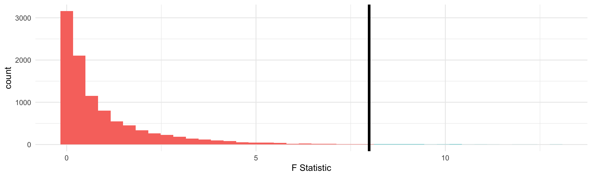
• The p-value calculates values “as extreme or more extreme”, in the t-distribution “more extreme values”, defined as farther from 0, can be positive or negative. Not so for the F!

Example

anova(mod)

Analysis of Variance Table

Response: leaf_length
           Df Sum Sq Mean Sq F value   Pr(>F)   
leaf_width  1  226.7  226.71  7.9882 0.005707 **
Residuals  98 2781.2   28.38                    
---
Signif. codes:  0 '***' 0.001 '**' 0.01 '*' 0.05 '.' 0.1 ' ' 1

summary(mod)

Call:
lm(formula = leaf_length ~ leaf_width, data = magnolia_data)

Residuals:
     Min       1Q   Median       3Q      Max 
-12.4544  -3.2196  -0.0287   3.1761  12.6086 

Coefficients:
            Estimate Std. Error t value Pr(>|t|)    
(Intercept)  11.8362     1.3956   8.481 2.36e-13 ***
leaf_width    0.4386     0.1552   2.826  0.00571 ** 
---
Signif. codes:  0 '***' 0.001 '**' 0.01 '*' 0.05 '.' 0.1 ' ' 1

Residual standard error: 5.327 on 98 degrees of freedom
Multiple R-squared:  0.07537,   Adjusted R-squared:  0.06593 
F-statistic: 7.988 on 1 and 98 DF,  p-value: 0.005707

• Notice the p-value for the F-test is the same as the p-value for the \(\hat\beta_1\) t-test
• This is always true for simple linear regression (with just one \(x\) variable)

What is the F-test testing?

anova(mod)

Analysis of Variance Table

Response: leaf_length
           Df Sum Sq Mean Sq F value   Pr(>F)   
leaf_width  1  226.7  226.71  7.9882 0.005707 **
Residuals  98 2781.2   28.38                    
---
Signif. codes:  0 '***' 0.001 '**' 0.01 '*' 0.05 '.' 0.1 ' ' 1

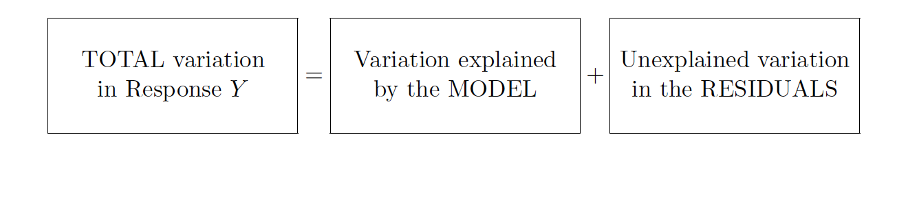
• null hypothesis: the fit of the intercept only model (with \(\hat\beta_0\) only) and your model (\(\hat\beta_0 + \hat\beta_1x\)) are equivalent
• alternative hypothesis: The fit of the intercept only model is significantly worse compared to your model
• When we only have one variable in our model, \(x\), the p-values from the F and t tests are going to be equivalent

Relating the F and the t

anova(mod)

Analysis of Variance Table

Response: leaf_length
           Df Sum Sq Mean Sq F value   Pr(>F)   
leaf_width  1  226.7  226.71  7.9882 0.005707 **
Residuals  98 2781.2   28.38                    
---
Signif. codes:  0 '***' 0.001 '**' 0.01 '*' 0.05 '.' 0.1 ' ' 1

summary(mod)

Call:
lm(formula = leaf_length ~ leaf_width, data = magnolia_data)

Residuals:
     Min       1Q   Median       3Q      Max 
-12.4544  -3.2196  -0.0287   3.1761  12.6086 

Coefficients:
            Estimate Std. Error t value Pr(>|t|)    
(Intercept)  11.8362     1.3956   8.481 2.36e-13 ***
leaf_width    0.4386     0.1552   2.826  0.00571 ** 
---
Signif. codes:  0 '***' 0.001 '**' 0.01 '*' 0.05 '.' 0.1 ' ' 1

Residual standard error: 5.327 on 98 degrees of freedom
Multiple R-squared:  0.07537,   Adjusted R-squared:  0.06593 
F-statistic: 7.988 on 1 and 98 DF,  p-value: 0.005707

2.826^2

[1] 7.986276

Application Exercise

1. Open appex-11.qmd
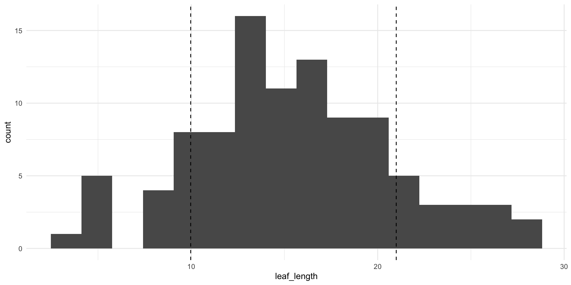
2. Using your magnolia data, predict leaf length from leaf width
3. What are the degrees of freedom for the: Sum of Squares Total, Sum of Squares Model, Sum of Squares Errors
4. Calculate the following quantities: Sum of Squares Total, Sum of Squares Model, Sum of Squares Errors
5. Calculate the F-statistic for the model and the p-value
6. What is the null hypothesis? What is the alternative?

06:00