Regression and Correlation

Lucy D’Agostino McGowan

Application Exercise

1. Copy the following template into RStudio Pro:

https://github.com/sta-112-f22/appex-12.git

2. Load the packages and then examine the PorschePrice data frame
3. Fit a linear model predicting a Porsche’s price from the mileage
4. Examine the ANOVA table – what is the F statistic? What is the associated p-value? Why hypothesis is it testing?

04:00

Partitioning variability

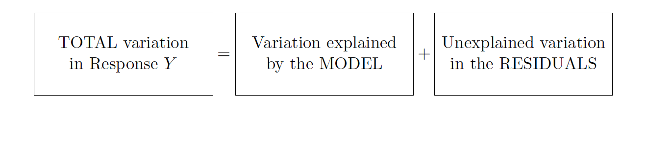
Why?

• \(y − \bar{y} = (\hat{y} − \bar{y}) + (y − \hat{y})\)
• \(\sum(y − \bar{y})^2 = \sum(\hat{y} − \bar{y})^2 + \sum(y − \hat{y})^2\)
  

• SSTotal = SSModel + SSE

coefficient of determination

Often referred to as \(\color{#86a293}{r^2}\), it is the fraction of the response variability that is explained by the model.

Coefficient of determination

• \(r^2 = \frac{\textrm{Variability explained by the model}}{\textrm{Total variability in } y}\)
• \(r^2 = \frac{\textrm{SSModel}}{\textrm{SSTotal}}\)
• \(r^2 = \frac{\sum(\hat{y} - \bar{y})^2}{\sum(y-\bar{y})^2}\)

Application Exercise

\[r^2 = \frac{\textrm{SSModel}}{\textrm{SSTotal}}\]

How could you calculate \(r^2\) if all you had was \(\textrm{SSTotal}\) and \(\textrm{SSE}\)?

01:00

Coefficient of determination

• \(r^2 = \frac{\textrm{Variability explained by the model}}{\textrm{Total variability in } y}\)
• \(r^2 = \frac{\textrm{SSModel}}{\textrm{SSTotal}}\)
• \(r^2 = \frac{\sum(\hat{y} - \bar{y})^2}{\sum(y-\bar{y})^2}\)

• \(r^2 = \frac{\textrm{SSTotal − SSE}}{\textrm{SSTotal}}\)
• \(r^2 = 1 - \frac{\textrm{SSE}}{\textrm{SSTotal}}\)

Let’s do it in R!

mod <- lm(leaf_length ~ leaf_width, data = magnolia_data)
summary(mod)

Call:
lm(formula = leaf_length ~ leaf_width, data = magnolia_data)

Residuals:
     Min       1Q   Median       3Q      Max 
-12.4544  -3.2196  -0.0287   3.1761  12.6086 

Coefficients:
            Estimate Std. Error t value Pr(>|t|)    
(Intercept)  11.8362     1.3956   8.481 2.36e-13 ***
leaf_width    0.4386     0.1552   2.826  0.00571 ** 
---
Signif. codes:  0 '***' 0.001 '**' 0.01 '*' 0.05 '.' 0.1 ' ' 1

Residual standard error: 5.327 on 98 degrees of freedom
Multiple R-squared:  0.07537,   Adjusted R-squared:  0.06593 
F-statistic: 7.988 on 1 and 98 DF,  p-value: 0.005707

7.5% of the variation in the length of a magnolia leaf is explained by it’s width.

Application Exercise

1. Open appex-12.qmd
2. Run summary on your model predicting Porsche price from mileage
3. What is the \(r^2\)? How can you interpret this?

03:00