Multiple linear regression

Confounder example

Confounder example

Confounder example

Confounder example
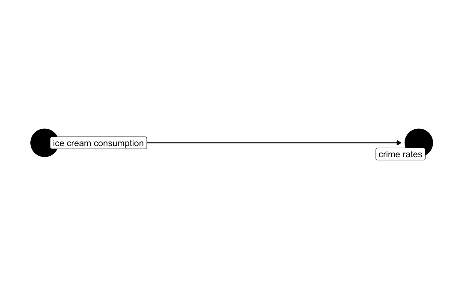
Confounder example
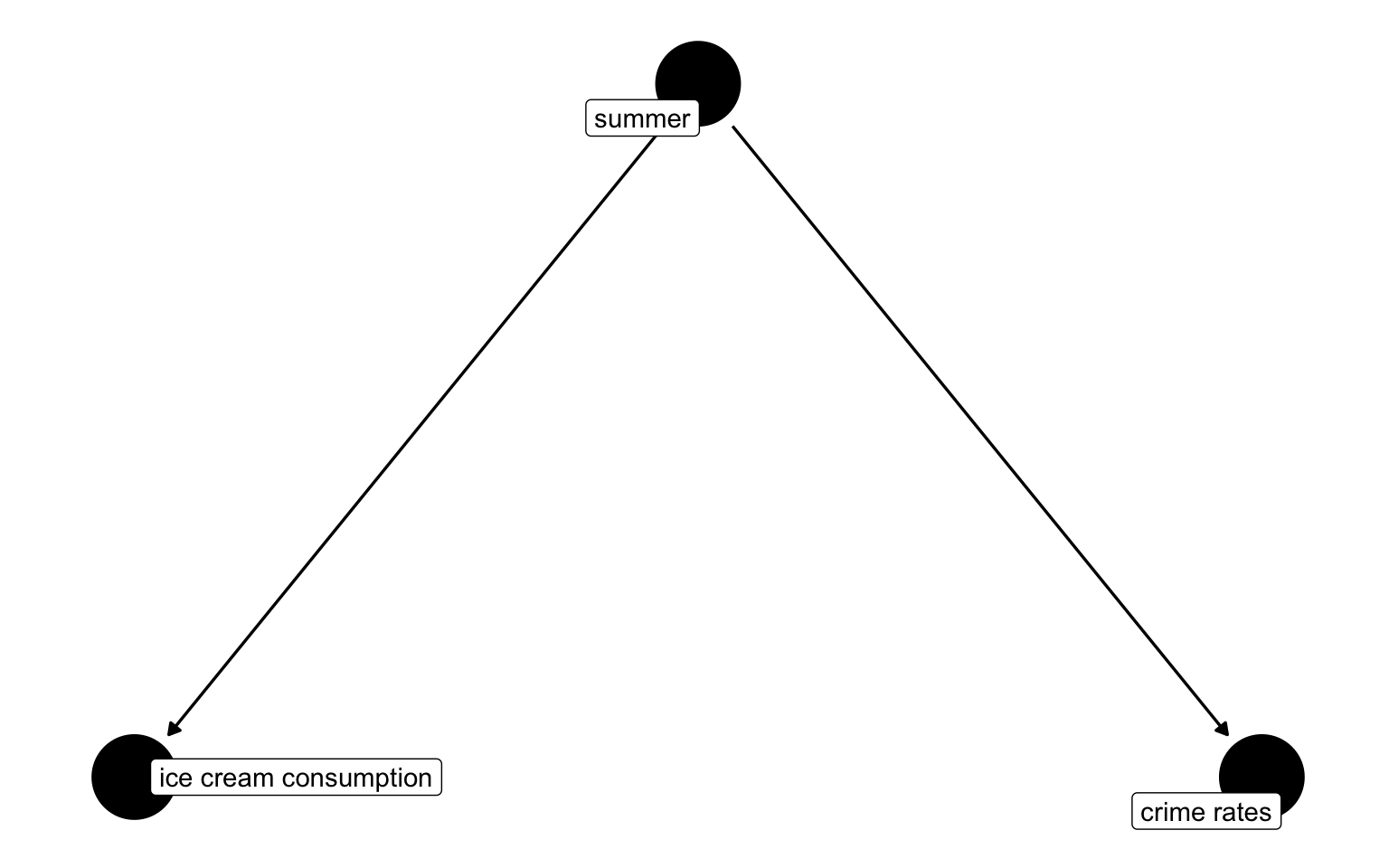
Confounding example
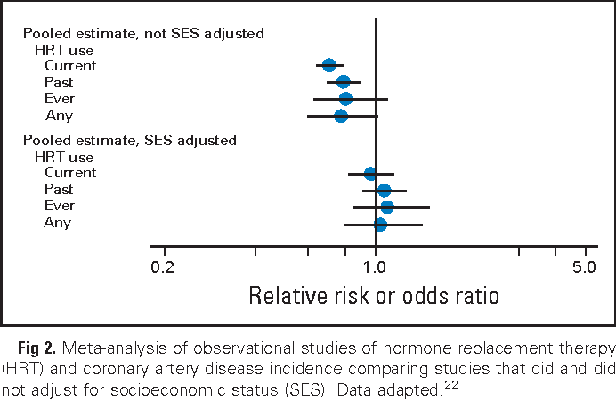
Armstrong, K.A. (2012). Methods in comparative effectiveness research. Journal of clinical oncology: official journal of the American Society of Clinical Oncology, 30 34, 4208-14.
Berkley administration data
- Study carried out by the graduate Division of the University of California, Berkeley in the early 70’s to evaluate whether there was a gender bias in graduate admissions
- The data come from six departments. For confidentiality we’ll call them A-F.
- We have information on whether the applicant was male or female and whether they were admitted or rejected.
- First, we will evaluate whether the percentage of males admitted is indeed higher than females, overall. Next, we will calculate the same percentage for each department.
![]() Slides adapted from datasciencebox.org by Dr. Lucy D’Agostino McGowan
Slides adapted from datasciencebox.org by Dr. Lucy D’Agostino McGowan
Simpson’s paradox
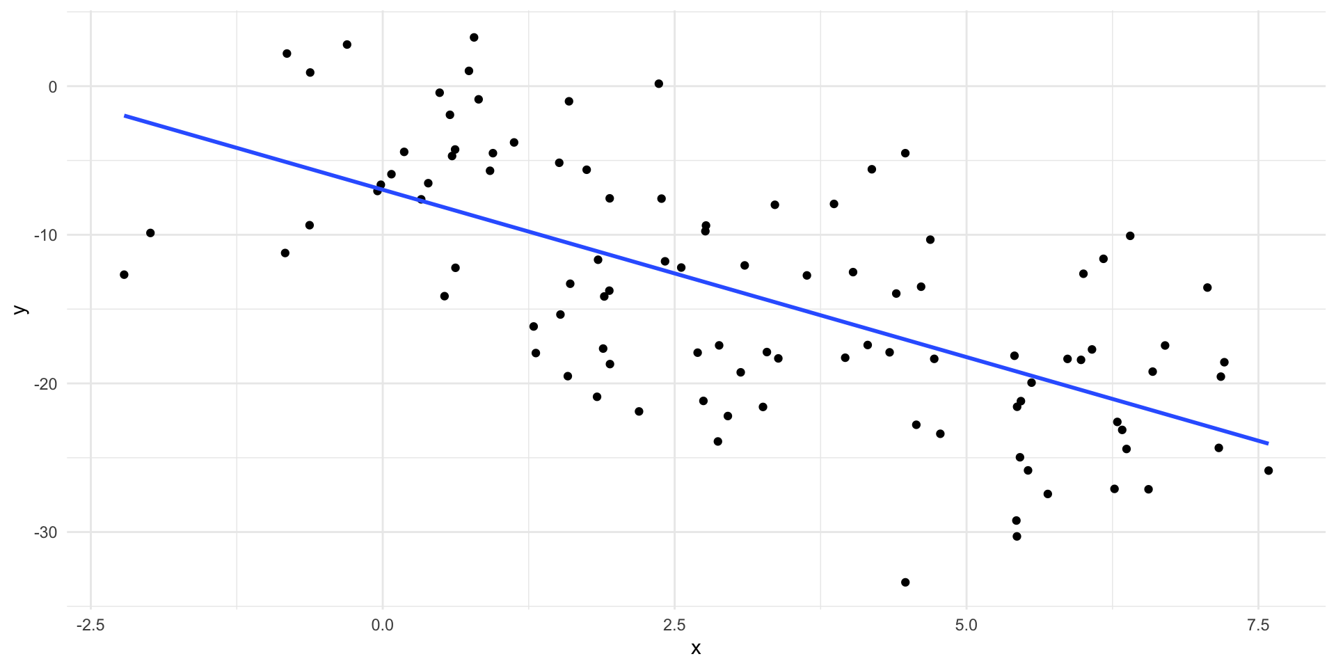
Simpson’s paradox
Code
set.seed(1)
data <- tibble(
  x = c(rnorm(25), rnorm(25, 2), rnorm(25, 4), rnorm(25, 6)),
  group = rep(1:4, each = 25),
  y = 5 + 2.5 * x - 10 * group + rnorm(100, 0, 5)
)
ggplot(data, aes(x, y, color = group)) +
  geom_point() +
  geom_smooth(method = "lm", formula = "y ~ x", se = FALSE, aes(group = group)) +
theme(legend.position = "none") 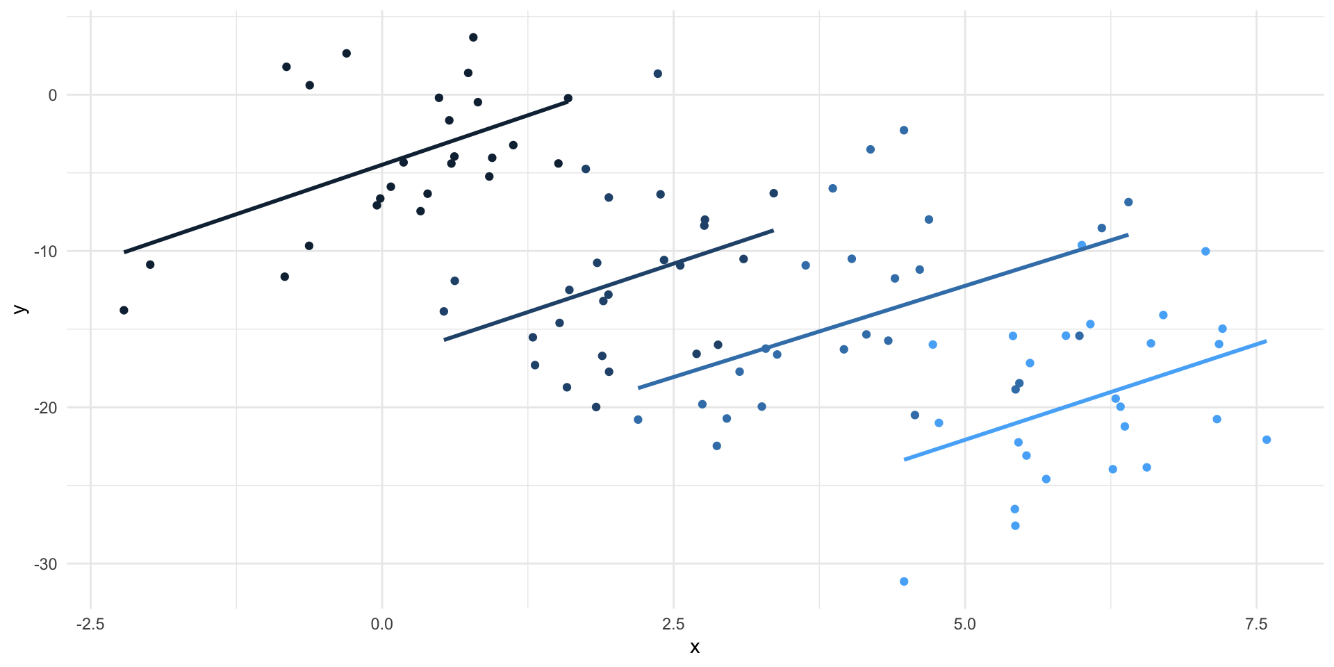
Application Exercise
Open
appex-13.qmdUsing the
NFL2007Standingsdata create a model that predictsWinPctfromPointsFor.Examine the \(R^2\) and \(R^2_{adj}\) values.Using the NFL2007Standings data create a model that predicts
WinPctfromPointsForANDPointsAgainst.Examine the \(R^2\) and \(R^2_{adj}\) values.Which model do you think is better for predicting win percent?
05:00
