What is the relationship between average SAT scores and average teacher salaries?
Are we doing inference or prediction?
Adjusting for confounders
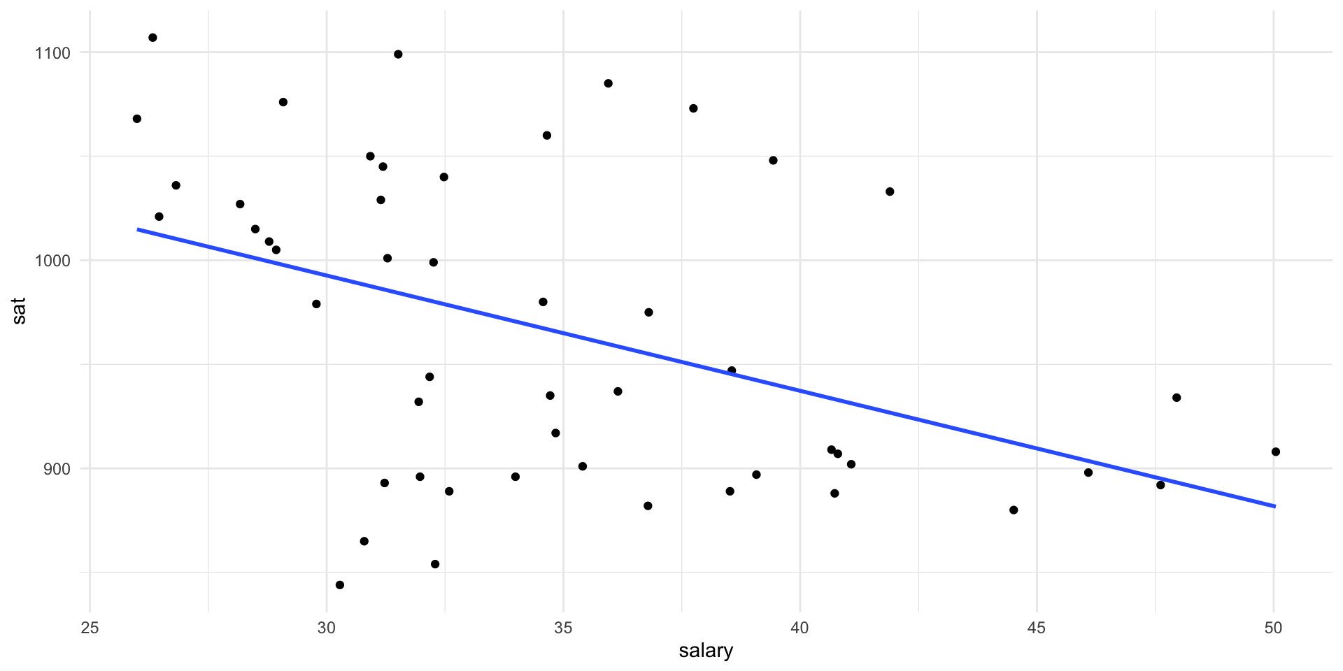
I fit a linear model for \(\hat{sat} = \hat\beta_0 + \hat\beta_1 salary\)
lm(sat ~ salary, SAT)
Call:
lm(formula = sat ~ salary, data = SAT)

Coefficients:
(Intercept)       salary
    1158.86        -5.54
How do we interpret this result?
Adjusting for confounders
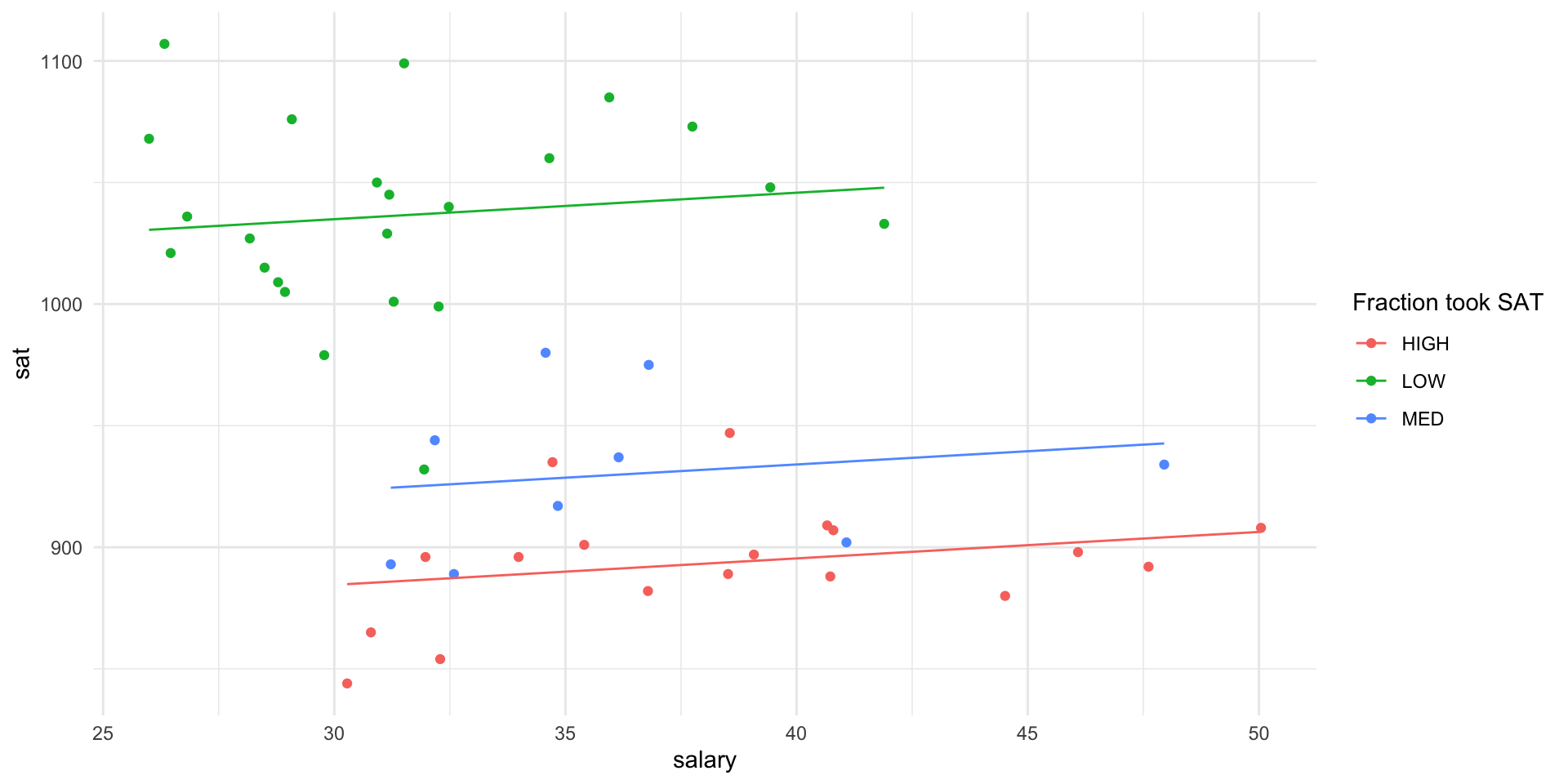
There is a third variable, the fraction of students that took the SAT in that state. It is grouped as “Low”, “Medium”, and, “High”.
Code
SAT <- SAT %>%mutate(frac_group =case_when( frac <22~"LOW", frac <49~"MED",TRUE~"HIGH" ))lm(sat ~ salary + frac_group, SAT)
Call:
lm(formula = sat ~ salary + frac_group, data = SAT)

Coefficients:
  (Intercept)         salary  frac_groupLOW  frac_groupMED
      851.866          1.089        150.379         38.636
What is the referent category?
How do you interpret the \(\hat{\beta}\) for frac_groupLOW?
How do you interpret the \(\hat{\beta}\) for salary now?
\(\hat\beta\) interpretation in multiple linear regression
The coefficient for \(x\) is \(\hat\beta\) (95% CI: \(LB_\hat\beta, UB_\hat\beta\)). A one-unit increase in \(x\) yields an expected increase in y of \(\hat\beta\), holding all other variables constant.
\(\hat\beta\) interpretation in multiple linear regression
The coefficient for average salary is 1.09 (95% CI: -0.90, 3.08). A $1,000 increase in average salary yields an expected increase in average SAT score of 1.09, holding the fraction of students that took the SAT constant.
Adjusting for confounders
Code
ggplot(SAT, aes(salary, sat)) +geom_point() +geom_smooth(method ="lm", se =FALSE)
Adjusting for confoundrs
Code
ggplot(SAT, aes(salary, sat, color = frac_group, group = frac_group)) +geom_point() +geom_line(aes(y =predict(lm(sat ~ salary + frac_group, data = SAT)))) +labs(color ="Fraction took SAT")
What is this called? Where the direction reverses?
Notice here the lines are parallel so holding the group constant, this is the effect we see.
😱 what if the lines aren’t parallel?
Interactions
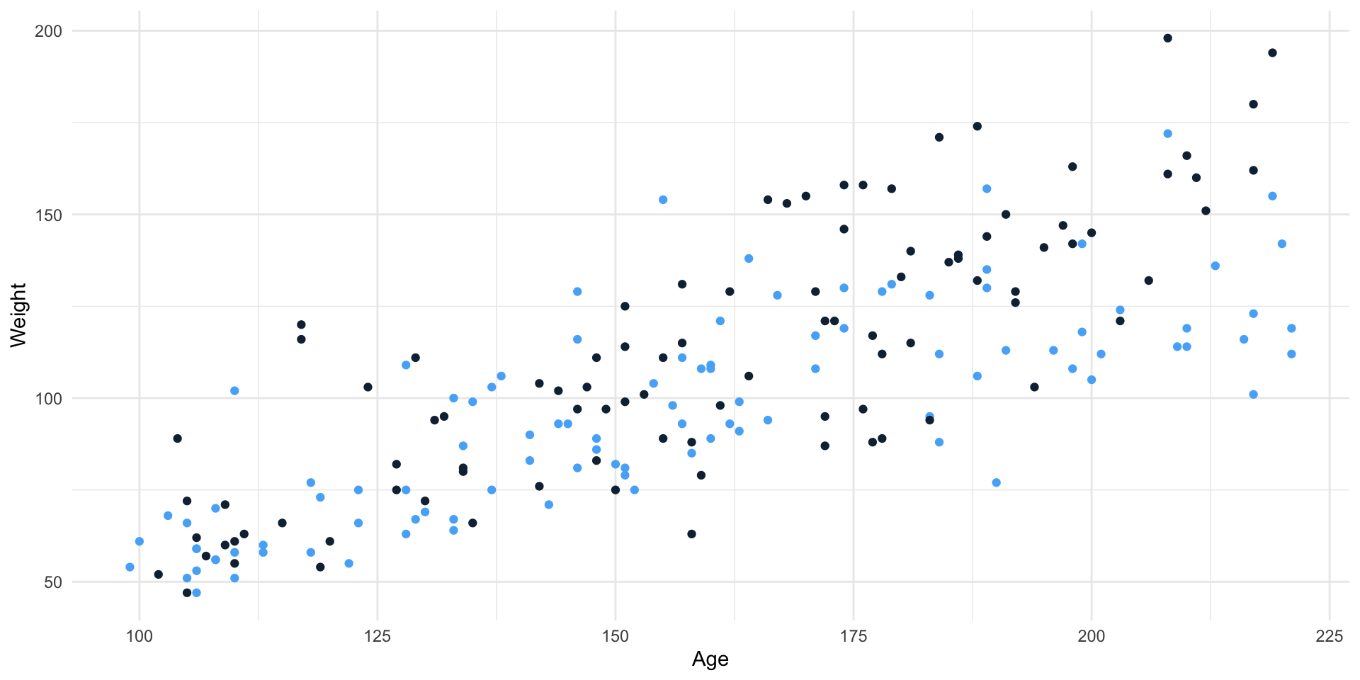
Data looking at the growth rate for kids
Interactions
Code
ggplot(Kids198, aes(Age, Weight)) +geom_point()
Will \(\hat\beta_{age}\) be positive or negative?
Interactions
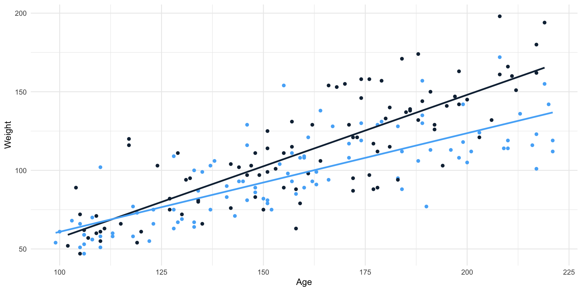
Let’s look at this relationship split by sex (blue: Girl, black: Boy)
Code
ggplot(Kids198, aes(Age, Weight, color = Sex)) +geom_point() +theme(legend.position ="none")
Interactions
Let’s look at this relationship split by sex (blue: Girl, black: Boy)
Code
ggplot(Kids198, aes(Age, Weight, color = Sex, group = Sex)) +geom_point() +theme(legend.position ="none") +geom_smooth(method ="lm", se =FALSE)
😱 the lines cross! That means there is an interaction, that is the slopes differ based on the group
Interactions
Let’s look at this relationship split by sex (blue: Girl, black: Boy)
Code
ggplot(Kids198, aes(Age, Weight, color = Sex, group = Sex)) +geom_point() +theme(legend.position ="none") +geom_smooth(method ="lm", se =FALSE)
What is the equation for this relationship?
Interactions
\(Weight = \beta_0 + \beta_1 Age + \beta_2 Girl + \beta_3 Age \times Girl + \epsilon\)
lm(Weight ~ Age + Sex + Age * Sex, data = Kids198)
Call:
lm(formula = Weight ~ Age + Sex + Age * Sex, data = Kids198)

Coefficients:
(Intercept)          Age          Sex      Age:Sex
   -33.6925       0.9087      31.8506      -0.2812
What does this model become for boys (When Sex = 0)
\(Weight = \beta_0 + \beta_1 Age + \epsilon\)
What does this model become for girls (When Sex = 1)
\(Weight = \beta_0 + \beta_1 Age + \beta_2 1 + \beta_3 Age \times 1 + \epsilon\)
How much the slope changes as we move from the regression line for boys to that for girls
Interactions
\(Weight = \beta_0 + \beta_1 Age + \beta_2 Girl + \beta_3 Age \times Girl + \epsilon\)
Hypothesis testing: What if you want to test whether the slope is different between groups?
Is the growth rate different for boys and girls?
What is \(H_0\)?
\(H_0: \beta_3 = 0\)
What is \(H_A\)?
\(H_A:\beta_3 \neq 0\)
Interactions
Code
lm(Weight ~ Age + Sex + Age * Sex, data = Kids198) %>%summary()
Call:
lm(formula = Weight ~ Age + Sex + Age * Sex, data = Kids198)

Residuals:
    Min      1Q  Median      3Q     Max
-46.884 -12.055  -2.782  10.185  58.581

Coefficients:
             Estimate Std. Error t value Pr(>|t|)
(Intercept) -33.69254   10.00727  -3.367 0.000917 ***
Age           0.90871    0.06106  14.882  < 2e-16 ***
Sex          31.85057   13.24269   2.405 0.017106 *
Age:Sex      -0.28122    0.08164  -3.445 0.000700 ***
---
Signif. codes:  0 '***' 0.001 '**' 0.01 '*' 0.05 '.' 0.1 ' ' 1

Residual standard error: 19.19 on 194 degrees of freedom
Multiple R-squared:  0.6683,    Adjusted R-squared:  0.6631
F-statistic: 130.3 on 3 and 194 DF,  p-value: < 2.2e-16
What is the result of our hypothesis test?
\(\hat\beta\) interpretation for interactions between \(x\) and a binary indicator \(I\)
The coefficient for the interaction between \(x\) and \(I\) is \(\hat\beta\) (95% CI: \(LB_\hat\beta, UB_\hat\beta\)). This means that the effect of \(x\) on \(y\) differs by \(\hat\beta\) when \(I = 1\) compared to \(I = 0\)holding all other variables constant*.
You must include this line if there are additional variables in your model.
\(\hat\beta\) interpretation for interactions between \(x\) and a binary indicator \(I\)
The coefficient for the interaction between Age and Sex is -0.28 (95% CI: -0.44, -0.12). This means that the expected effect of Age on Weight is lower by 0.28 among girls compared to boys.
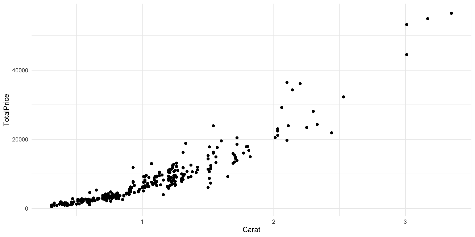
Non-linear relationships
Sometimes the relationships between the outcome \(y\) and \(x\) variables are nonlinear.
We can use polynomials to address this!
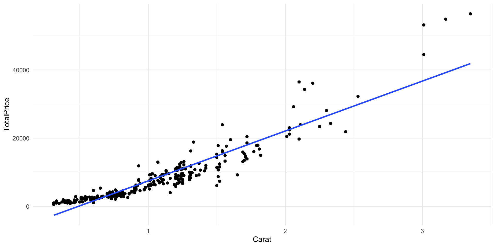
Returning to the Diamonds data, let’s say we are interested in predicting Total Price from the Carats.
Typically, in multiple linear regression, the interpretation of \(\hat\beta_i\) is: a one-unit change in \(x\) yields an expected change in \(y\) of \(\hat\beta_i\)holding all other variables constant.
What does it mean to see a change in Caret holding Carat\(^2\) constant?
When you have a polynomial term, you need to specify the values you are changing between, since the change is no longer constant across all values of \(x\).
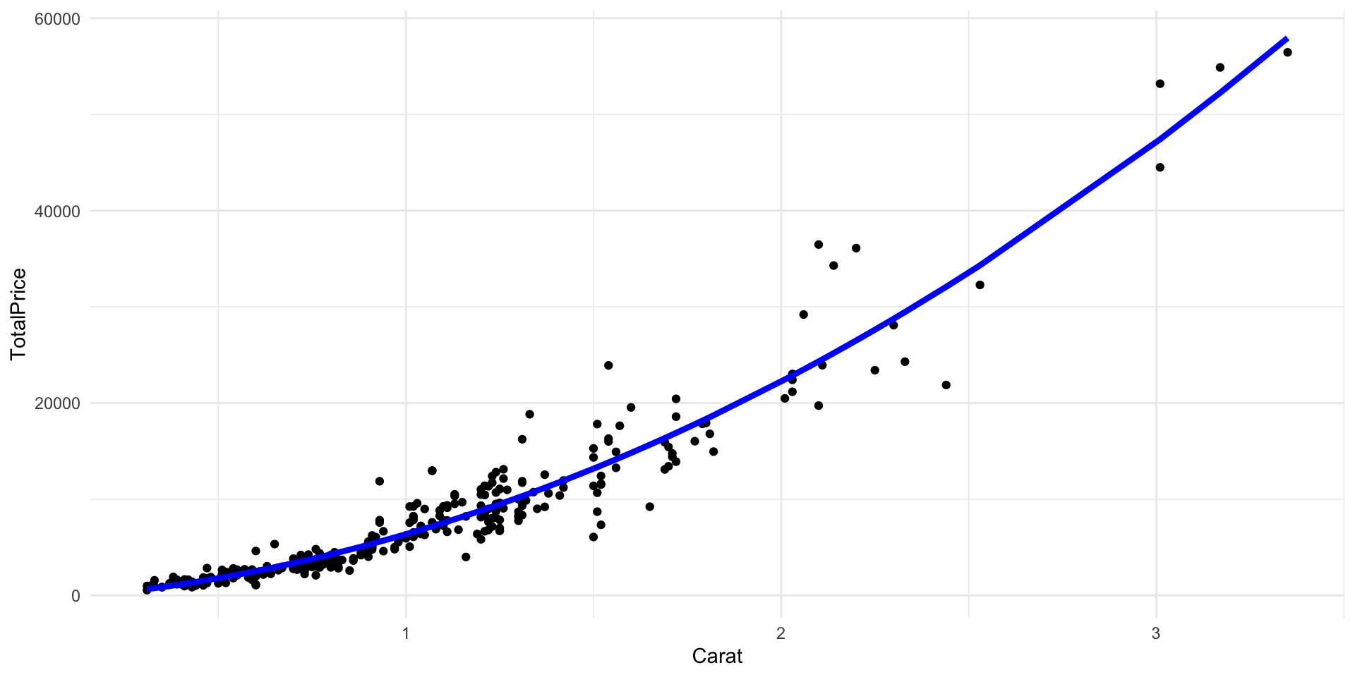
Interpreting \(\hat\beta\) in the presence of polynomials
lm(TotalPrice ~ Carat +I(Carat^2), data = Diamonds)
What is the expected change in TotalPrice for a one-unit change in Carat, changing from 1.8 to 2.8?
2386* (2.8-1.8) +4498.2* (2.8^2-1.8^2)
[1] 23077.72
Can we talk about \(\hat\beta_1\) and \(\hat\beta_2\) in the context of a one-unit change in Carat?
Interpreting \(\hat\beta\) in the presence of polynomials
\(\hat\beta\) coefficients that are transformations of the same \(x\) variable must be interpreted together
You must first choose to values of \(x\) to change between, and then report the change.
A sensible choice for the two \(x\) values can be the 25th% quantile and the 75th% quantile.
General \(\hat\beta\) interpretation with quadratic terms
The linear term in the model for \(x\) has a coefficient of \(\hat\beta_1\) (95% CI: \((LB_{\hat\beta_1}, UB_{\hat\beta_1})\)). The quadratic term in the model for \(x\) has a coefficient of \(\hat\beta_2\) (95% CI: \((LB_{\hat\beta_2}, UB_{\hat\beta_2})\)). A change in \(x\) from \(a\) to \(b\) yields an expected change in \(y\) of \(\hat\beta_1 (b - a) + \hat\beta_2 (b^2 - a^2)\)holding all other variables constant*.
You must include this line if there are additional variables in your model.
Specific \(\hat\beta\) interpretation for \(y = \beta_0 + \beta_1 Carat + \beta_2 Carat^2 + \epsilon\) model
The linear term in the model for Carat has a coefficient of 2386 (95% CI: \((906, 3866)\)). The quadratic term in the model for Carat has a coefficient of \(4498\) (95% CI: \((3981, 5016)\)). A change in Carat from \(0.7\) to \(1.24\) yields an expected change in TotalPrice of \(6000.5\).
Why didn’t I say holding all other variables constant?
Take aways
The interpretation of \(\hat\beta\) in multiple linear regression
A one-unit change in \(x\) yields an expected change in \(y\) of \(\hat\beta\)holding all other included variables constant
If the slope differs between groups (the lines cross in a scatterplot), an interaction is present
You can include polynomial terms to address non-linear relationships
The coefficients for a polynomial must be interpreted together
`Application Exercise}
Open appex-14.qmd
Fit the model \(TotalPrice = \beta_0 + \beta_1Carat + \beta_2 Carat^2 + \beta_3 Color+\epsilon\)
Find the 0.25 quantile and 0.75 quantile of Carat
What is the interpretation of \(\hat\beta_1\), \(\hat\beta_2\), and \(\hat\beta_3\)?