Evaluating Multiple Linear Regression Models
Marginal effect plots
Marginal effect plots
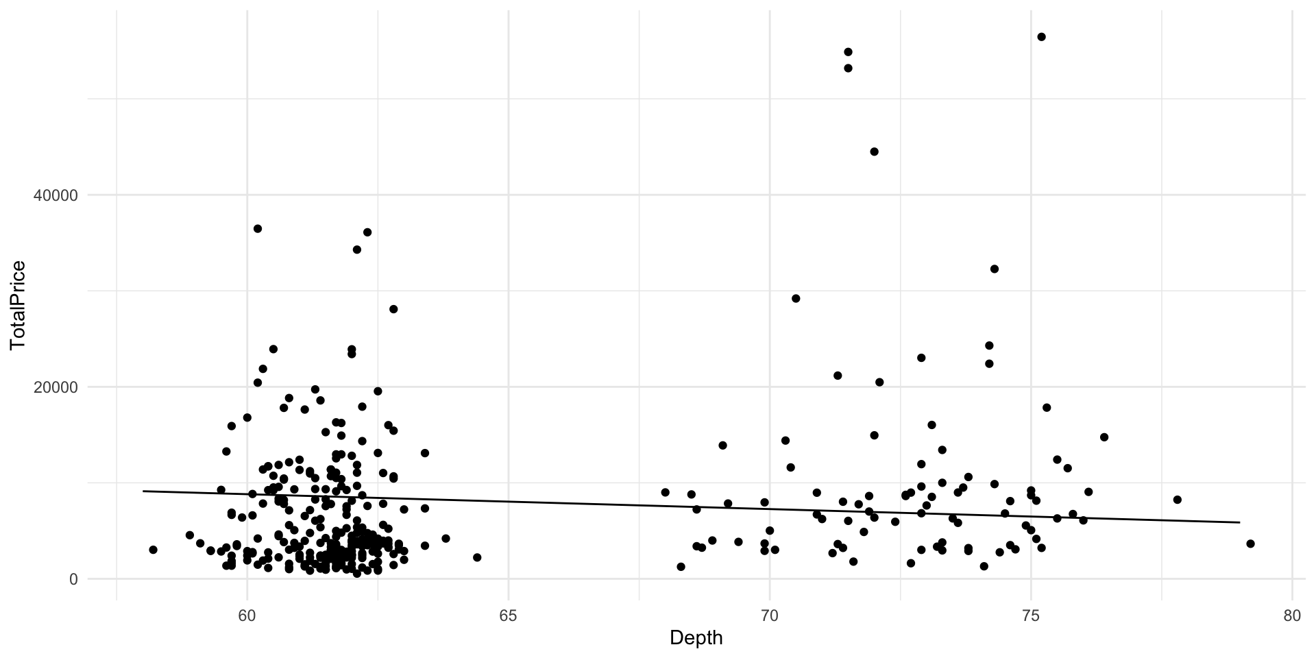
Marginal effect plots
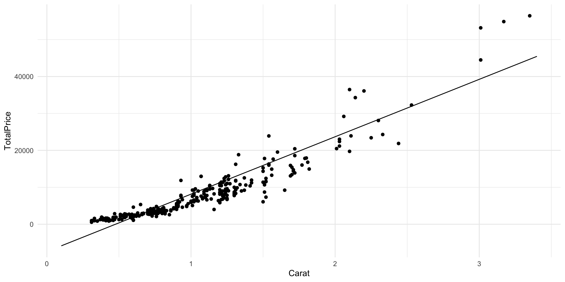
Transformation of y example
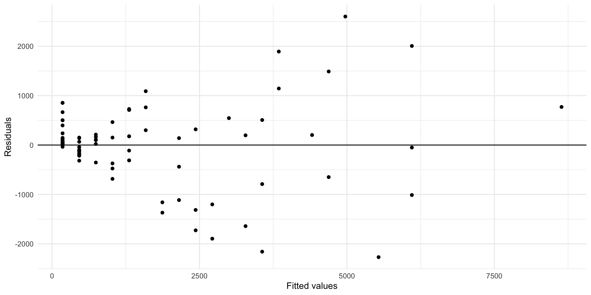
Transformation of y example
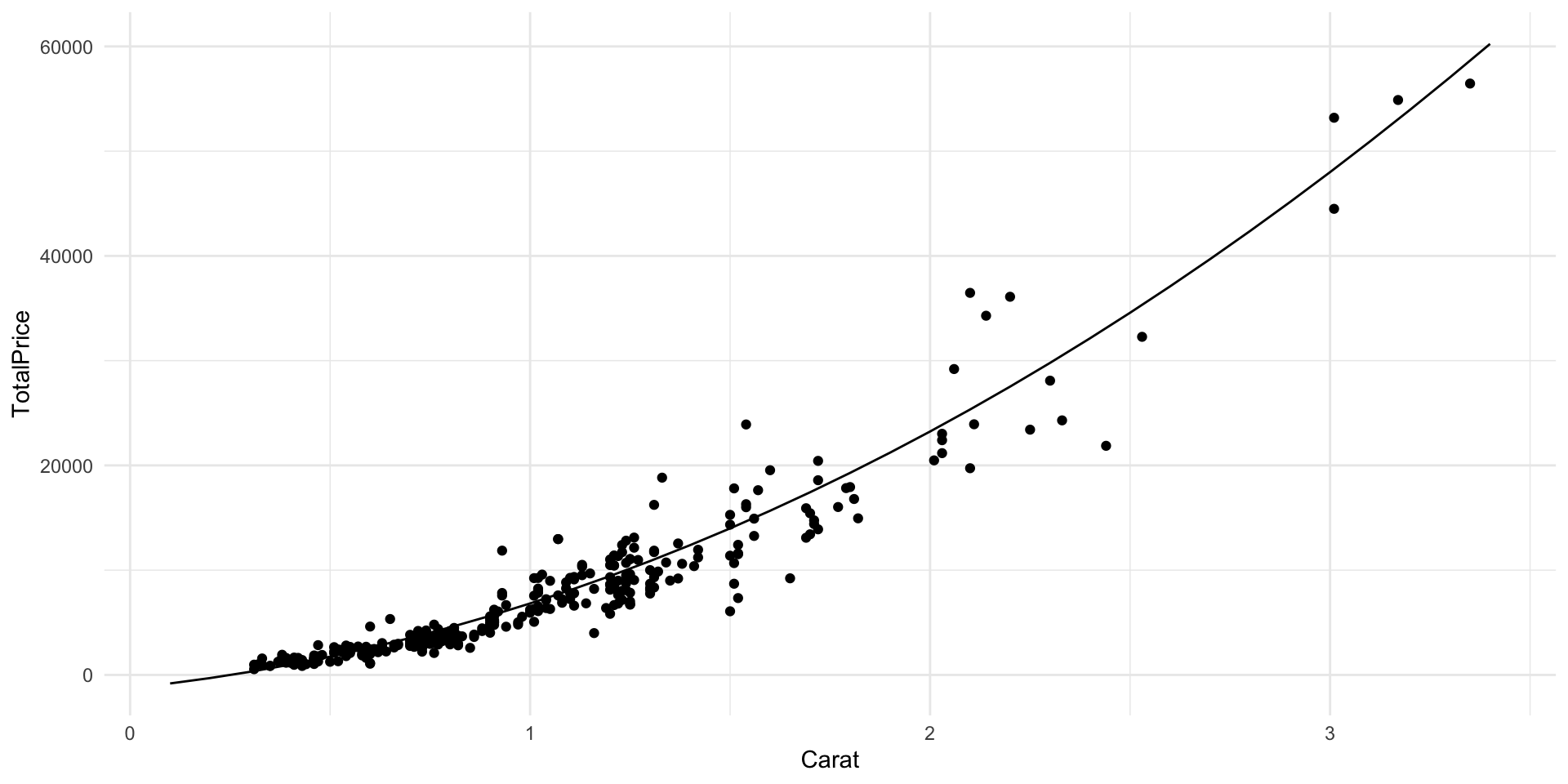
Try taking the log of the outcome.
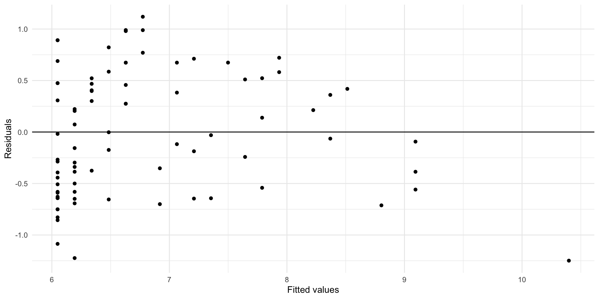
Transformation of y example
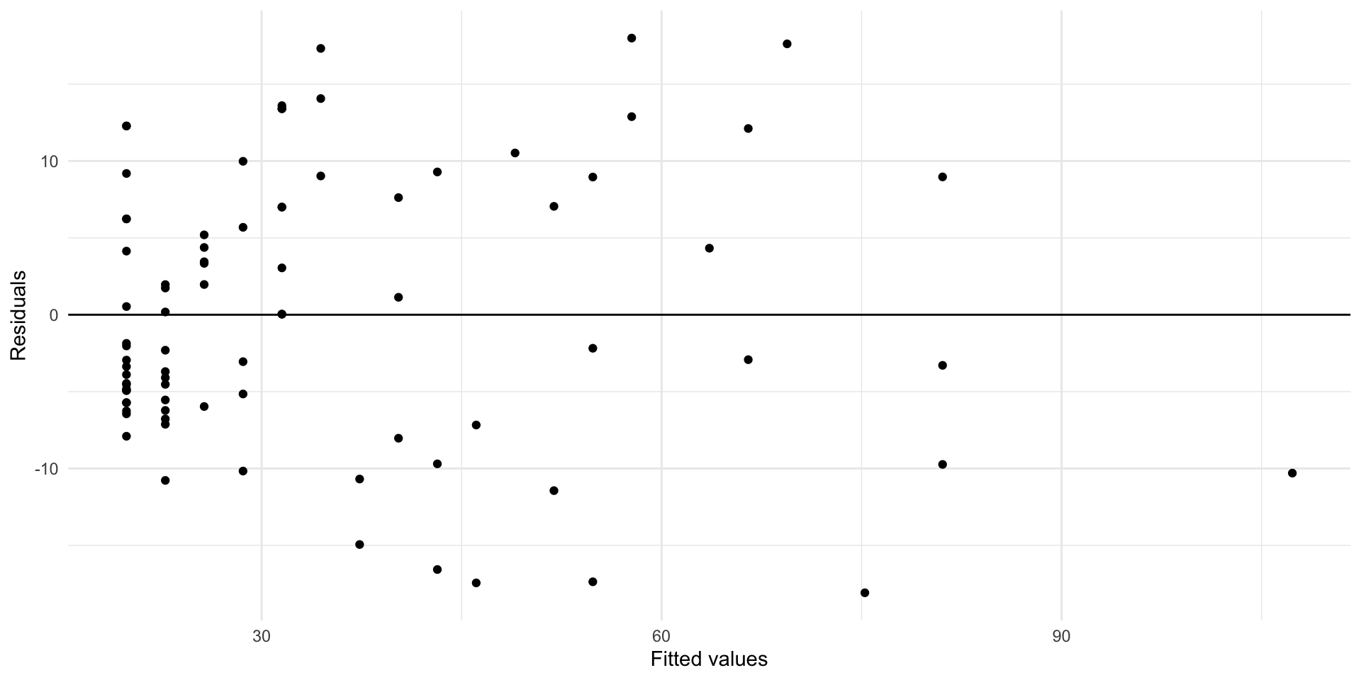
Try taking the square root of the outcome.
Conditions for multiple linear regression
| Assumption | What it means | How do you check? | How do you fix? |
|---|---|---|---|
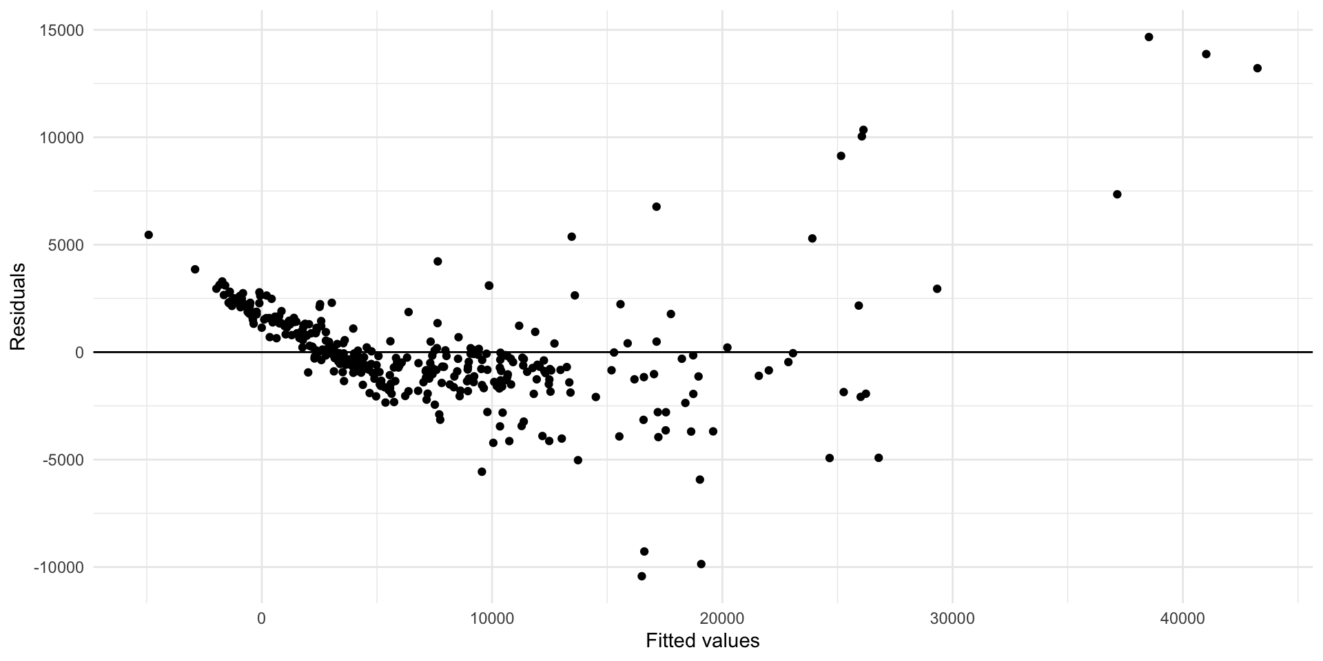
| Linearity | The relationship between the outcome and explanatory variable or predictor is linear holding all other variables constant | Residuals vs. fits plot Marginal effects plots |
fit a better model (transformations, polynomial terms, more / different variables, etc.) |
| Zero Mean | The error distribution is centered at zero | by default | – |
| Constant Variance | The variability in the errors is the same for all values of the predictor variable | Residuals vs fits plot | fit a better model (try taking the log or square root of the outcome) |
| Independence | The errors are assumed to be independent from one another | 👀 data generation | Find better data or fit a fancier model |
| Random | The data are obtained using a random process | 👀 data generation | Find better data |
| Normality | The random errors follow a normal distribution | QQ-plot / residual histogram | fit a better model |
