Selecting predictors

Lucy D’Agostino McGowan

Selecting variables

When the goal is inference how do we choose what to include in our model?

• We need to understand the theoretical relationship between the explanatory variable we are interested in, the outcome variable we are interested in, and any confounders.
• There is not a statistical test we can do to test whether we have included all relevant variables

Selecting variables

• When the goal is prediction we can use the metrics we learned about last class to compare models
• But how do we choose what to put in those models to begin with?
• What if we look at every combination of all available variables?

Multicollinearity

• One concern with including every potential combination of all variables is that we may include variables that are highly correlated
• In the extreme case, if one predictor has an exact linear relationship with one ormore other predictors in the model, the least squares process does not have a unique solution

d <- tibble(
  x1 = rnorm(100),
  x2 = rnorm(100),
  x3 = 3 * x1 + 4 * x2,
  y = rnorm(100)
)

lm(y ~ x1 + x2 + x3, data = d)

Call:
lm(formula = y ~ x1 + x2 + x3, data = d)

Coefficients:
(Intercept)           x1           x2           x3  
    0.12514      0.03661     -0.02821           NA  

Multicollinearity

• In the less extreme case where the variables are not perfect linear combinations of each other, but still highly correlated, including all variables could inflate your variance

Code

set.seed(1)
d <- tibble(
  x1 = rnorm(100),
  x2 = rnorm(100),
  x3 = 4 * x2 + rnorm(100, sd = 0.1),
  y = x1 + x2 + rnorm(100)
)

summary(lm(y ~ x1 + x2 + x3, data = d))

Call:
lm(formula = y ~ x1 + x2 + x3, data = d)

Residuals:
     Min       1Q   Median       3Q      Max 
-2.58201 -0.52738  0.00281  0.65058  1.82364 

Coefficients:
            Estimate Std. Error t value Pr(>|t|)    
(Intercept)  0.05273    0.10065   0.524    0.602    
x1           0.94204    0.11169   8.434  3.4e-13 ***
x2          -3.23987    3.88095  -0.835    0.406    
x3           1.04623    0.97118   1.077    0.284    
---
Signif. codes:  0 '***' 0.001 '**' 0.01 '*' 0.05 '.' 0.1 ' ' 1

Residual standard error: 0.998 on 96 degrees of freedom
Multiple R-squared:  0.6144,    Adjusted R-squared:  0.6024 
F-statistic:    51 on 3 and 96 DF,  p-value: < 2.2e-16

Code

summary(lm(y ~ x1 + x2, data = d))

Call:
lm(formula = y ~ x1 + x2, data = d)

Residuals:
     Min       1Q   Median       3Q      Max 
-2.48809 -0.54939 -0.05717  0.65489  1.81422 

Coefficients:
            Estimate Std. Error t value Pr(>|t|)    
(Intercept)  0.05538    0.10070   0.550    0.584    
x1           0.94425    0.11177   8.448 2.96e-13 ***
x2           0.93946    0.10480   8.964 2.31e-14 ***
---
Signif. codes:  0 '***' 0.001 '**' 0.01 '*' 0.05 '.' 0.1 ' ' 1

Residual standard error: 0.9989 on 97 degrees of freedom
Multiple R-squared:  0.6098,    Adjusted R-squared:  0.6017 
F-statistic: 75.79 on 2 and 97 DF,  p-value: < 2.2e-16

• Here, I am focusing on the \(\hat\beta\) and it’s standard error, is this an inference focus or prediction?

Multicollinearity

• For prediction we care about multicollinearity if we are trying to fit a parsimonious model. We can potentially remove predictors that are highly correlated with other variables since they don’t add much additional information
• To determine how correlated a predictor is with all of the other variables included, we can examine the variance inflation factor

\[VIF_i = \frac{1}{1-R_i^2}\]

• \(R_i^2\) is the \(R^2\) value from the model used to predict \(X_i\) from all of the remaining predictors.

Variance inflation factor

summary(lm(x1 ~ x2 + x3, data = d))

Call:
lm(formula = x1 ~ x2 + x3, data = d)

Residuals:
     Min       1Q   Median       3Q      Max 
-2.30129 -0.60350  0.01765  0.58513  2.27806 

Coefficients:
            Estimate Std. Error t value Pr(>|t|)
(Intercept)  0.10841    0.09083   1.194    0.236
x2          -0.63849    3.52738  -0.181    0.857
x3           0.15960    0.88270   0.181    0.857

Residual standard error: 0.9073 on 97 degrees of freedom
Multiple R-squared:  0.0003379, Adjusted R-squared:  -0.02027 
F-statistic: 0.01639 on 2 and 97 DF,  p-value: 0.9837

1 / (1 - 0.0003379)

[1] 1.000338

summary(lm(x2 ~ x1 + x3, data = d))

Call:
lm(formula = x2 ~ x1 + x3, data = d)

Residuals:
      Min        1Q    Median        3Q       Max 
-0.066055 -0.016015  0.000616  0.011195  0.073233 

Coefficients:
              Estimate Std. Error t value Pr(>|t|)    
(Intercept) -0.0006617  0.0026323  -0.251    0.802    
x1          -0.0005288  0.0029217  -0.181    0.857    
x3           0.2501524  0.0006856 364.880   <2e-16 ***
---
Signif. codes:  0 '***' 0.001 '**' 0.01 '*' 0.05 '.' 0.1 ' ' 1

Residual standard error: 0.02611 on 97 degrees of freedom
Multiple R-squared:  0.9993,    Adjusted R-squared:  0.9993 
F-statistic: 6.657e+04 on 2 and 97 DF,  p-value: < 2.2e-16

1 / (1 - 0.9993)

[1] 1428.571

• A rule of thumb is that we suspect multicollinearity if VIF > 5
• We could drop one of the highly correlated predictors from our model

Choosing predictors

• We could try every combination of all variables
• This could get computationally expensive - you are fitting \(2^k\) models (so if you have 10 predictors, that is 1,024 models you are choosing between, yikes!)
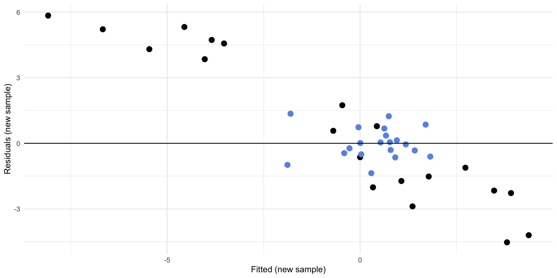
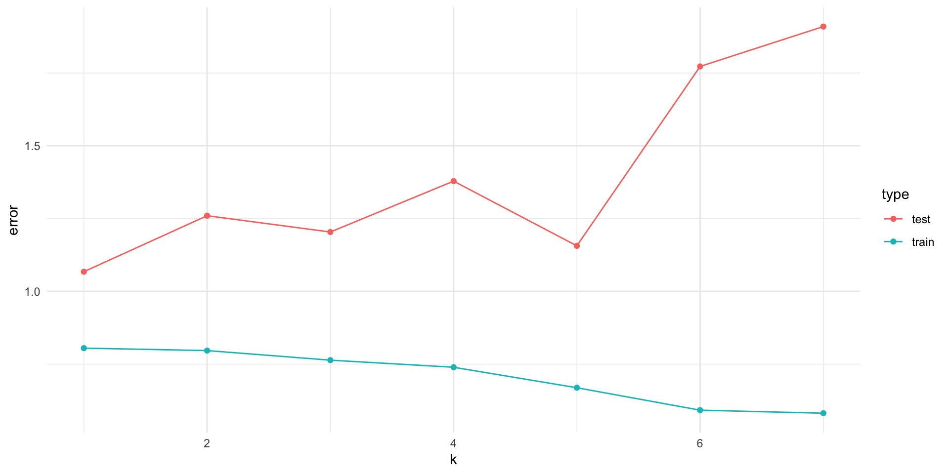
• Another issue with trying every possible combination of models is you could overfit your model to your data – that is, the model might fit very well to these particular observations, but would do a poor job predicting a new sample.

Overfitting

Code

set.seed(1)
d_samp1 <- tibble(
  x1 = rnorm(20),
  x2 = rnorm(20),
  x3 = rnorm(20),
  x4 = rnorm(20),
  x5 = rnorm(20),
  x6 = rnorm(20),
  x7 = rnorm(20),
  x8 = rnorm(20),
  x9 = rnorm(20),
  x10 = rnorm(20),
  x11 = rnorm(20),
  x12 = rnorm(20),
  x13 = rnorm(20),
  x14 = rnorm(20),
  x15 = rnorm(20),
  y = x1 + rnorm(20)
)

set.seed(98)
d_samp2 <- tibble(
  x1 = rnorm(20),
  x2 = rnorm(20),
  x3 = rnorm(20),
  x4 = rnorm(20),
  x5 = rnorm(20),
  x6 = rnorm(20),
  x7 = rnorm(20),
  x8 = rnorm(20),  
  x9 = rnorm(20),
  x10 = rnorm(20),
  x11 = rnorm(20),
  x12 = rnorm(20),
  x13 = rnorm(20),
  x14 = rnorm(20),
  x15 = rnorm(20),
  y =  x1 + rnorm(20)
)

mod <- lm(y ~ x2 + x3 + x4 + x5 + x6 + x7 + x8 + x9 + x10 + x11 + x12 + x13 + x14 + x15, data = d_samp1)
summary(mod)

Call:
lm(formula = y ~ x2 + x3 + x4 + x5 + x6 + x7 + x8 + x9 + x10 + 
    x11 + x12 + x13 + x14 + x15, data = d_samp1)

Residuals:
       1        2        3        4        5        6        7        8 
-0.64403 -0.45154 -0.04833 -0.60674  1.24050  0.73453  0.04043  0.67753 
       9       10       11       12       13       14       15       16 
 1.35489  0.01393  0.85657 -0.30261 -1.36512 -0.98604 -0.32717  0.35345 
      17       18       19       20 
-0.22440  0.05106 -0.50264  0.13574 

Coefficients:
            Estimate Std. Error t value Pr(>|t|)
(Intercept)  -0.4426     0.6120  -0.723    0.502
x2            0.3862     0.9031   0.428    0.687
x3            1.8937     1.0206   1.856    0.123
x4           -0.3759     0.7050  -0.533    0.617
x5           -1.0079     0.8513  -1.184    0.290
x6            1.0262     1.1077   0.926    0.397
x7            1.0259     0.7000   1.466    0.203
x8           -0.3547     0.5261  -0.674    0.530
x9            0.5444     0.6198   0.878    0.420
x10           1.1507     1.2804   0.899    0.410
x11          -0.1104     0.4339  -0.254    0.809
x12          -1.1195     0.6272  -1.785    0.134
x13          -0.6836     0.8355  -0.818    0.450
x14           1.5101     1.2347   1.223    0.276
x15           1.1414     1.1929   0.957    0.383

Residual standard error: 1.384 on 5 degrees of freedom
Multiple R-squared:  0.6546,    Adjusted R-squared:  -0.3126 
F-statistic: 0.6768 on 14 and 5 DF,  p-value: 0.7413

Code

ggplot(d_samp1, aes(x = fitted(mod), y = residuals(mod))) +
  geom_point(size = 3) +
  geom_hline(yintercept = 0) +
  labs(x = "Fitted value",
       y = "Residuals")

Overfitting

mean(residuals(mod)^2)

[1] 0.4790626

resids <- d_samp2$y - predict(mod, d_samp2)
resids

         1          2          3          4          5          6          7 
 4.7286669  5.3216536  5.2166364 -0.6350207 -1.1162105 -2.2761892  4.5665798 
         8          9         10         11         12         13         14 
-2.8854733 -4.5302358  0.7835241  1.7420493  4.3076951 -1.5185146  3.8490034 
        15         16         17         18         19         20 
-2.1626190 -1.7239860  5.8441660  0.5729056 -4.2033428 -2.0147232 

mean(resids^2)

[1] 11.88054

Code

ggplot(d_samp2, aes(x = predict(mod, d_samp2), y = resids)) +
  geom_point(size = 3) + 
  geom_point(aes(x = fitted(mod), y = residuals(mod)), color = "cornflower blue", size = 3) + 
  geom_hline(yintercept = 0) + 
  labs(x = "Fitted (new sample)",
       y = "Residuals (new sample)")

Overfitting

• Solution: Fit the model on part of the data and calculate the error on the remaining part
• Cross-validation: fit the model on a subset of observations, see how it performs on the rest
• Leave-on-out cross validation: fit the model on n-1 observations, see how the model performs on the nth

LOOCV

set.seed(10)
train <- d_samp1 %>%
  sample_n(19)
test <- d_samp1 %>%
  anti_join(train)
mod <- lm(y ~ x1 + x2 + x3 + x4 + x5 + x6 + x7 + x8 + x9 + x10 + x11 + x12 + x13 + x14 + x15, data = train)
summary(mod)

Call:
lm(formula = y ~ x1 + x2 + x3 + x4 + x5 + x6 + x7 + x8 + x9 + 
    x10 + x11 + x12 + x13 + x14 + x15, data = train)

Residuals:
       1        2        3        4        5        6        7        8 
 0.21045 -0.23308 -0.12596  0.42737  0.02388 -0.30874  0.26494  0.27812 
       9       10       11       12       13       14       15       16 
 0.04443 -0.33224 -0.02625  0.22471  0.03455  0.14295  0.23164 -0.21622 
      17       18       19 
-0.10781 -0.33574 -0.19699 

Coefficients:
            Estimate Std. Error t value Pr(>|t|)  
(Intercept) -1.29965    0.49820  -2.609   0.0798 .
x1           3.61723    1.15476   3.132   0.0520 .
x2           0.39510    0.38179   1.035   0.3768  
x3           1.47738    0.43120   3.426   0.0417 *
x4           2.45737    0.92006   2.671   0.0756 .
x5           0.07084    0.43470   0.163   0.8809  
x6           1.39491    0.54188   2.574   0.0822 .
x7           0.10954    0.43321   0.253   0.8167  
x8          -0.20495    0.22021  -0.931   0.4207  
x9           0.20127    0.27177   0.741   0.5126  
x10          4.46902    1.53815   2.905   0.0622 .
x11          0.28387    0.33111   0.857   0.4543  
x12          0.14482    0.44312   0.327   0.7653  
x13         -1.85182    0.48823  -3.793   0.0322 *
x14          4.44539    1.39637   3.184   0.0500 *
x15          3.04203    1.07255   2.836   0.0658 .
---
Signif. codes:  0 '***' 0.001 '**' 0.01 '*' 0.05 '.' 0.1 ' ' 1

Residual standard error: 0.5742 on 3 degrees of freedom
Multiple R-squared:  0.9611,    Adjusted R-squared:  0.7667 
F-statistic: 4.944 on 15 and 3 DF,  p-value: 0.1068

mean(residuals(mod)^2)

[1] 0.05206743

mean((test$y - predict(mod, test))^2)

[1] 19.44538

LOOCV

Code

get_error <- function(k) {
  train <- d_samp1 %>%
    sample_n(19)
  test <- d_samp1 %>%
    anti_join(train, by = c("x1", "x2", "x3", "x4", "x5", "x6", "x7", "y"))
  form <- as.formula(glue(
    "y ~ {glue_collapse(glue('x{1:k}'), sep = ' + ')}"
  ))
  mod <- lm(form, data = train)
  tibble(
    error = c(mean(residuals(mod)^2), mean((test$y - predict(mod, test))^2)),
    type = c("train", "test"),
    k = k
  )
}

set.seed(1)
err <- map_df(rep(1:7, each = 100), get_error) 
err %>%
  group_by(k, type) %>%
  summarise(error = mean(error)) %>%
  ggplot(aes(x = k, y = error, color = type)) +
  geom_point() +
  geom_line()

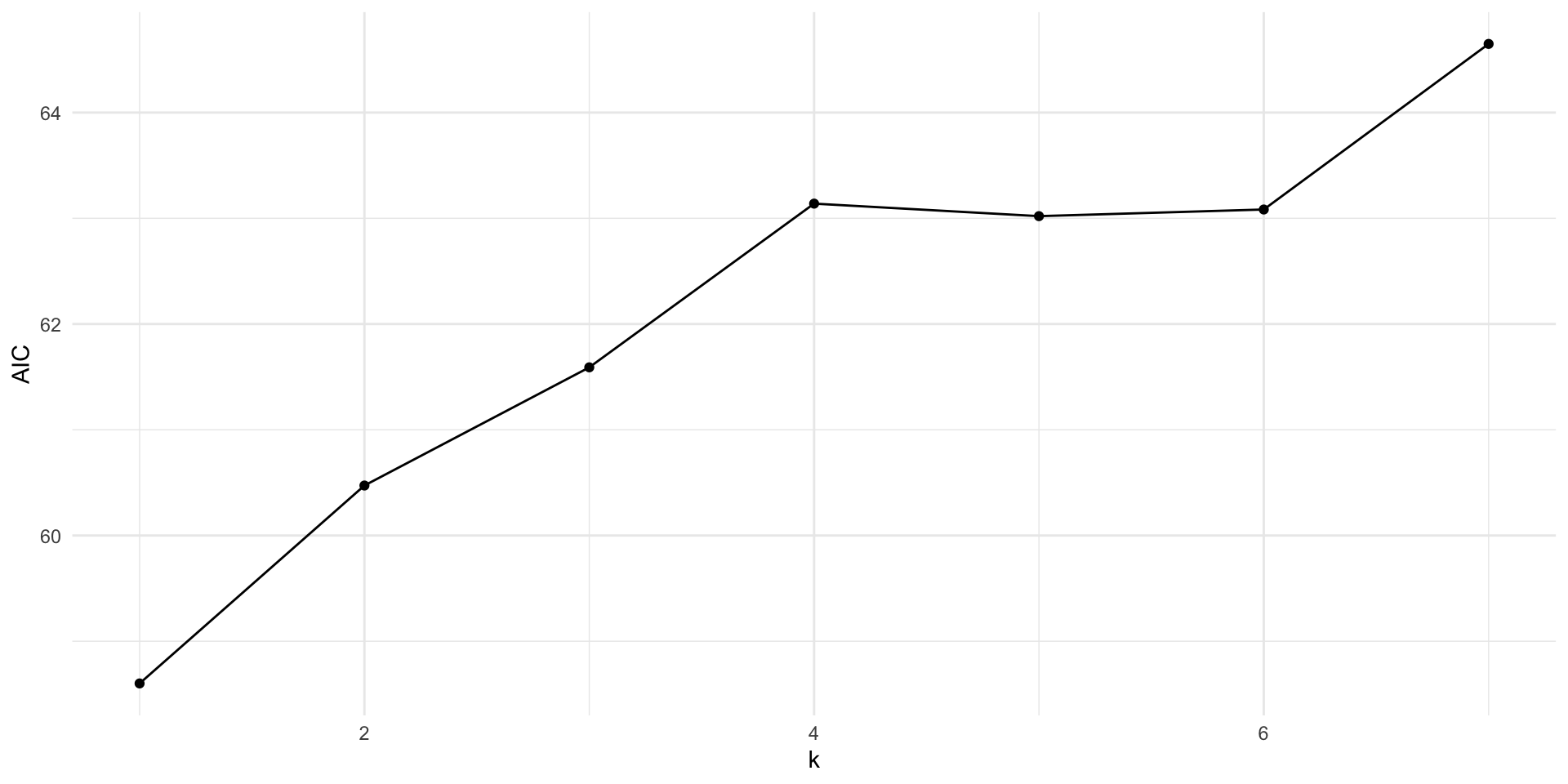
AIC

• It turns out in the case of linear regression, AIC mimics the choice from LOOCV so you don’t have to learn how to do this complicated method!

Code

get_aic <- function(k) {
   form <- as.formula(glue(
    "y ~ {glue_collapse(glue('x{1:k}'), sep = ' + ')}"
  ))
  mod <- lm(form, data = d_samp1)
  tibble(
    AIC = AIC(mod),
    k = k
  )
}

err <- map_df(1:7, get_aic)
err %>%
  ggplot(aes(x = k, y = AIC)) +
  geom_point() +
  geom_line()

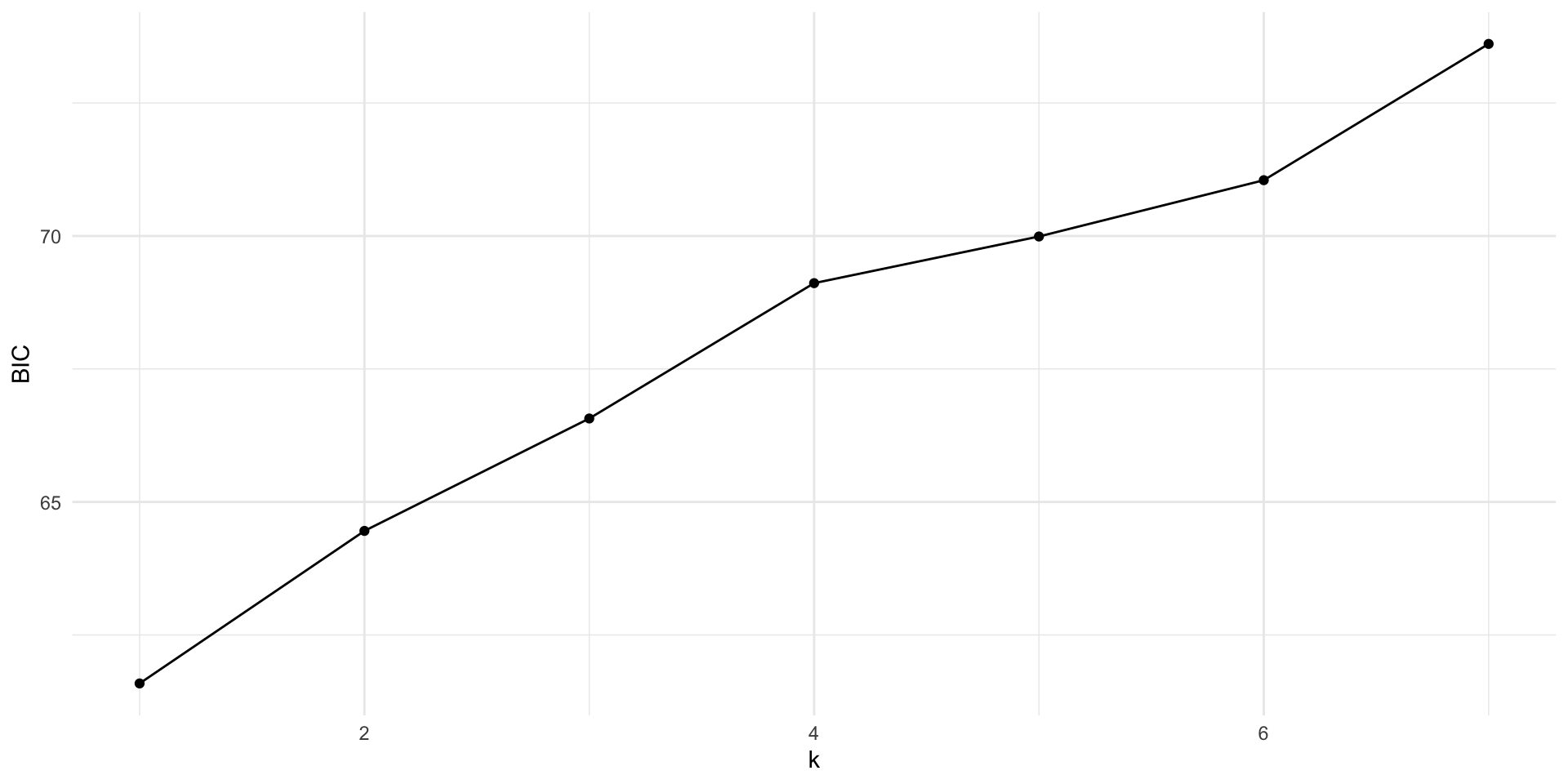
BIC

• BIC is equivalent to leave-\(k\)-out cross validation (where \(k = n[1-1/log(n)-1])\)) for linear models, so we can also use this metric without having to code up the complex cross validation!

Code

get_bic <- function(k) {
   form <- as.formula(glue(
    "y ~ {glue_collapse(glue('x{1:k}'), sep = ' + ')}"
  ))
  mod <- lm(form, data = d_samp1)
  tibble(
    BIC = BIC(mod),
    k = k
  )
}

err <- map_df(1:7, get_bic)
err %>%
  ggplot(aes(x = k, y = BIC)) +
  geom_point() +
  geom_line()

Big picture

inference

we need to use our theoretical understanding of the relationship between variables in order to properly select variables to include in our model

Big picture

inference

we need to use our theoretical understanding of the relationship between variables in order to properly select variables to include in our model

prediction

1. Choose a set of predictors to assess
2. Use a metric that balances parsimony with goodness of fit (\(R^2_{adj}\), AIC, BIC) to select the model
3. Best practice is to fit the model on one set of data and test it on another (using something like Leave-one-out cross validation), but it turns out AIC and BIC mimic this for linear regression (yay!) so we can reliably use these metric even when not splitting our data