Code
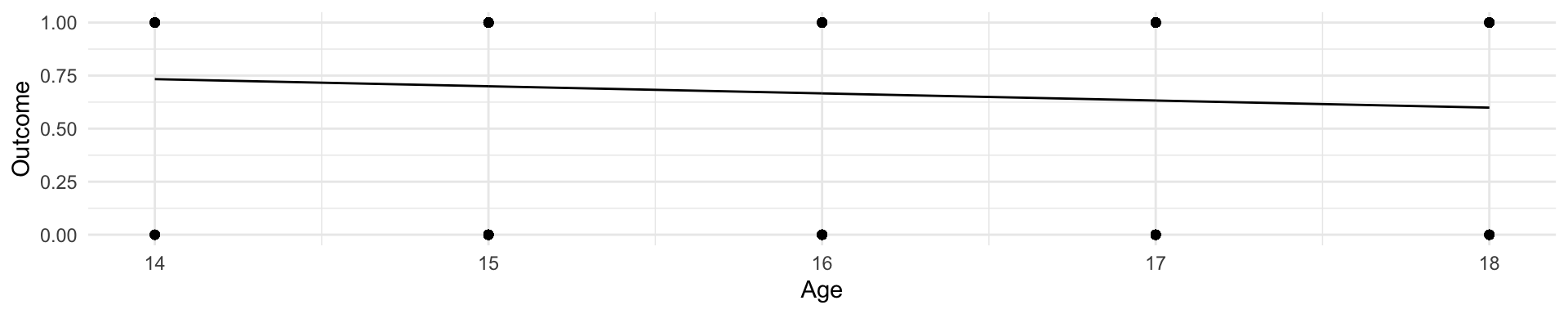
new_data <- data.frame(Age = 0:40)
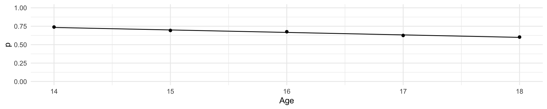
LosingSleep %>%
group_by(Age) %>%
count(Age, Outcome) %>%
mutate(p = n / sum(n)) %>%
filter(Outcome == 1) %>%
ggplot(aes(Age, p)) +
geom_point() +
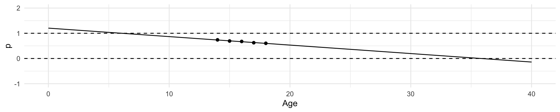
geom_line(data = new_data, aes(x = Age, y = predict(lm(Outcome ~ Age, data = LosingSleep), newdata = new_data))) +
ylim(-1, 2) +
xlim(0, 40) +
geom_hline(yintercept = c(0, 1), lty = 2) LosingSleep %>%
group_by(Age) %>%
count(Age, Outcome) %>%
mutate(p = n / sum(n)) %>%
filter(Outcome == 1) %>%
ggplot(aes(Age, p)) +
geom_point() +
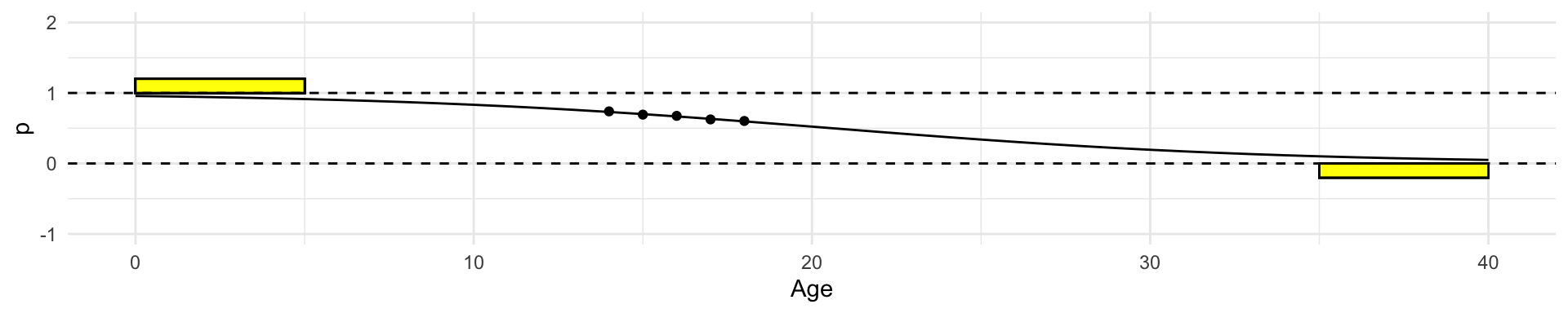
geom_rect(aes(xmin = 0, xmax = 5, ymin = 1, ymax = 1.2), fill = "yellow", color = "black") +
geom_rect(aes(xmin = 35, xmax = 40, ymin = 0, ymax = -0.2), fill = "yellow", color = "black") +
geom_line(data = new_data, aes(x = Age, y = predict(lm(Outcome ~ Age, data = LosingSleep), newdata = new_data))) +
ylim(-1, 2) +
xlim(0, 40) +
geom_hline(yintercept = c(0, 1), lty = 2) LosingSleep %>%
group_by(Age) %>%
count(Age, Outcome) %>%
mutate(p = n / sum(n)) %>%
filter(Outcome == 1) %>%
ggplot(aes(Age, p)) +
geom_point() +
geom_rect(aes(xmin = 0, xmax = 5, ymin = 1, ymax = 1.2), fill = "yellow", color = "black") +
geom_rect(aes(xmin = 35, xmax = 40, ymin = 0, ymax = -0.2), fill = "yellow", color = "black") +
geom_line(data = new_data,
aes(x = Age, y = predict(
glm(Outcome ~ Age, family = "binomial", data = LosingSleep),
newdata = new_data,
type = "response"))) +
ylim(-1, 2) +
xlim(0, 40) +
geom_hline(yintercept = c(0, 1), lty = 2) LosingSleep %>%
group_by(Age) %>%
count(Age, Outcome) %>%
mutate(p = n / sum(n)) %>%
filter(Outcome == 1) %>%
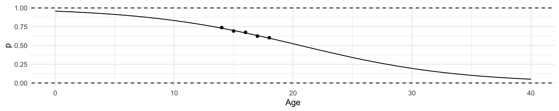
ggplot(aes(Age, p)) +
geom_point() +
geom_line(data = new_data,
aes(x = Age, y = predict(
glm(Outcome ~ Age, family = "binomial", data = LosingSleep),
newdata = new_data,
type = "response"))) +
xlim(0, 40) +
geom_hline(yintercept = c(0, 1), lty = 2) 1 2 3 4 5 6 7
0.63124876 0.85036851 0.16944765 0.71491359 0.31617156 0.74706022 0.88186412
8 9 10 11 12 13 14
0.27099332 0.73661581 0.88186412 0.92030775 0.45723876 0.79506038 0.61846455
15 16 17 18 19 20 21
0.23009846 0.52528952 0.66845438 0.52528952 0.18535740 0.88186412 0.73661581
22 23 24 25 26 27 28
0.79506038 0.89276358 0.87606259 0.70366831 0.55238896 0.39074729 0.57918073
29 30 31 32 33 34 35
0.34021444 0.83595184 0.63124876 0.08681729 0.88186412 0.72589836 0.17726253
36 37 38 39 40 41 42
0.86372477 0.52528952 0.34021444 0.87001815 0.11101432 0.30449919 0.31617156
43 44 45 46 47 48 49
0.63124876 0.90745180 0.30449919 0.29307306 0.92030775 0.06749390 0.22057873
50 51 52 53 54 55
0.69217046 0.01247874 0.55238896 0.44373791 0.01917403 0.39074729