Assumptions of Logistic Regression
⛳ Testing for linearity in logistic regression
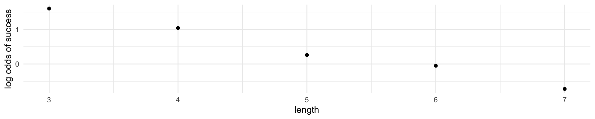
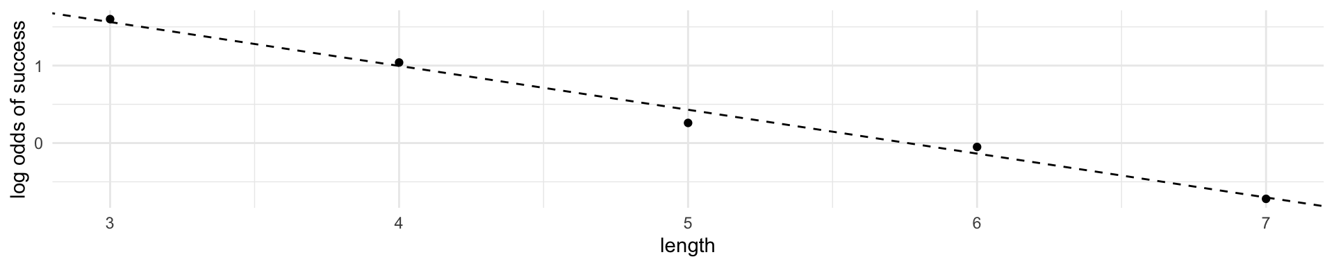
⛳ Testing for linearity in logistic regression
Testing for linearity in logistic regression
What if the \(x\) variable isn’t discrete?
- We can plot the empirical logit to examine the linearity assumption
- You can create “bins” and calculate the empirical logit within each bin (for example, count the number of success when x is between 1 and 5: bin 1, count the number of successes when x is between 5 and 10: bin 2, etc)
